%matplotlib inline
import numpy as np
import torch
import matplotlib.pyplot as plt
import plotting as P           # the course palette, the house style, and the figure helpers

torch.manual_seed(0);01 — What is Control? States, Controls, Targets and Feedback
Mathematical Foundations of Control and Machine Learning — Winter 2026
Central question. What does it mean mathematically to act on a dynamical system?
This notebook makes the vocabulary of the course precise — state, control, target, feedback — compares the three basic control questions.
Table of Contents
- A short history — from Ktesibios’s water clock to the state-space revolution
- The ingredients of a control problem — state equation, admissible controls, objective
- Three different questions — optimal control, controllability, stabilization; open and closed loop
- The overdamping paradox — energy decays faster, the state returns slower
- Control ↔︎ ML: two forward connections — reinforcement learning and momentum
- Exercises
# RK4 integrator for x' = f(t, x) along the time grid ts
def odeint(f, x0, ts):
    xs = [x0]
    for t, t1 in zip(ts[:-1], ts[1:]):
        x, h = xs[-1], t1 - t
        k1 = f(t, x)
        k2 = f(t + h / 2, x + h / 2 * k1)
        k3 = f(t + h / 2, x + h / 2 * k2)
        k4 = f(t + h, x + h * k3)
        xs.append(x + h / 6 * (k1 + 2 * k2 + 2 * k3 + k4))
    return torch.stack(xs)
Where are we?
A system has a state that evolves in time, we act on it through a control, and we want to reach a target. Here we make these words precise, compare the three basic control questions, and study the first example where intuition about control fails, the overdamped oscillator.
1. A short history
In the third century BCE, Ktesibios’s water clock used a float valve to keep its water supply steady — and antiquity already saw automation as a source of freedom, in a passage of Aristotle’s Politics. Windmills used fantails to turn into the wind automatically. In 1788, James Watt fitted a centrifugal governor to a steam engine: as two rotating balls moved outward, they adjusted a valve that controlled the steam supply. These devices worked, but a general mathematical account of their stability came later.
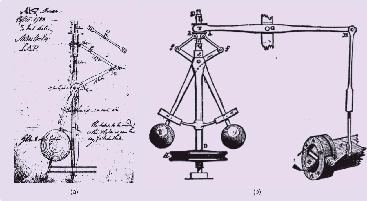
By the 1860s, engineers faced a practical problem: making a governor more responsive could cause it to oscillate, or hunt. In On Governors (1868), James Clerk Maxwell described small departures from steady operation with linear differential equations. He related stability to the roots of a characteristic polynomial: disturbances die away when every root has a negative real part — §4 works out the simplest instance of his analysis. In 1907, H. R. Hall stressed that regulators need fluctuations, which should be diminished but not removed.
In the 1920s–1930s, feedback entered telecommunications at the Bell Laboratories, and automatic control spread rapidly, along two parallel approaches: state space (ODEs) and frequency domain (Fourier). In 1948, N. Wiener named the field in Cybernetics, “the science of control and communication in animals and machines”.
In the 1950s and early 1960s, Bellman’s dynamic programming, Pontryagin’s maximum principle (a far-reaching generalization of Lagrange multipliers) and Kalman’s work on optimal control established modern state-space control. Kalman developed the concepts of controllability and observability and analyzed the linear–quadratic regulator using a Riccati equation. His 1960 paper on filtering addressed a different task — estimating a system’s state from noisy measurements — and was later used in Apollo’s onboard navigation. The theory then grew towards nonlinear, stochastic and infinite-dimensional (PDE) systems, with applications from acoustics and quantum control to aerospace, biomedicine and energy.
2. The ingredients of a control problem
A state equation describes how the state evolves and where we can act. For most cases, we consider a system of ordinary differential equations (ODEs) of the form \[ x'(t)=f\big(x(t),u(t)\big),\quad t\in(0,T),\qquad x(0)=x^0, \] where \(x(t)\in\mathbb R^n\) is the state to be controlled and \(u(t)\in\mathbb R^m\) is the control, taken from a set of admissible controls \(\mathcal U_{ad}\). Typical choices are \(\mathcal U_{ad}=L^2(0,T;\mathbb R^m)\) or controls with bounds, \(|u(t)|\le1\).
The same framework covers very different models: linear or nonlinear, deterministic or stochastic, finite- or infinite-dimensional, ordinary or partial differential equations, as well as hybrid models.
Example (the harmonic oscillator). The oscillator with a force, \(x_1''+x_1=u\), becomes a first-order system for \(x=(x_1,x_2)=(\text{position},\text{velocity})\): \[ x'=\begin{pmatrix}0&1\\-1&0\end{pmatrix}x+\begin{pmatrix}0\\1\end{pmatrix}u=A\,x+B\,u . \] It has one control acting on a two-dimensional state.
3. Three different questions
Several kinds of control problems fit the same framework, depending on how the objective is formulated.
Controllability. Given \(x^0\), \(x^1\) and \(T\), is there \(u\in\mathcal U_{ad}\) such that \(x(T)=x^1\) exactly? This is a more dynamical notion. The relaxed version, approximate controllability, asks for \(|x(T)-x^1|\le\varepsilon\) for every \(\varepsilon>0\).
Optimal control. Choose \(u\in\mathcal U_{ad}\) to minimize a cost, for example the distance to the target, or that distance plus the effort spent: \[ \min_{u\in\mathcal U_{ad}}\ J(u),\qquad J(u)=|x(T)-x^1|^2+\alpha\int_0^T|u(t)|^2dt . \] The answer is an optimal control. It need not reach the target: it makes the best compromise allowed by the cost.
Stabilization (feedback control). Find a rule \(u=F(x)\) such that every solution of the closed-loop system \[ x'=f\big(x,F(x)\big) \] tends to an equilibrium. The control is computed in real time from the state.
The last question introduces a distinction that runs through the whole course. A control can be
- open loop, \(u=u(t)\): a function of time, computed in advance from the model and then applied blindly;
- closed loop or feedback, \(u=F(x(t))\): computed in real time from the current state, so it can react to disturbances the model does not know about.
4. The overdamping paradox
The model. Without friction, the linearized pendulum \(x_1''+x_1=0\) conserves its energy \[ e(t)=\tfrac12\big(x_1(t)^2+x_1'(t)^2\big). \] With friction proportional to the velocity, \[ x_1''+x_1=-kx_1',\qquad k>0 . \] The control is \(u=-kx_2\) with a feedback law where the control opposes the measured velocity.
Energy decreases. Along solutions, \[ e'(t)=x_1x_1'+x_1'x_1''=x_1'\,(x_1+x_1'')=-k\,(x_1')^2\;\le\;0 . \] So more damping removes energy faster at each instant, for the same velocity. Does it follow that a larger \(k\) always brings the system to rest faster?
ks = [0.5, 1.0, 2.0, 4.0, 8.0]
x0 = torch.tensor([1.0, 0.0])
ts15 = torch.linspace(0, 15, 1501)

sols = {}
for k in ks:
    A_k = torch.tensor([[0.0, 1.0], [-1.0, -k]])       # the oscillator under the feedback u = -k x2
    sols[k] = odeint(lambda t, x: A_k @ x, x0, ts15)

shades = plt.cm.viridis(np.linspace(0, 0.85, len(ks)))
fig, (ax1, ax2) = P.panels(2, size=(4.3, 3.2))
for (k, x), c in zip(sols.items(), shades):
    ax1.plot(ts15, x[:, 0], color=c, label=f"$k={k:g}$")
    ax2.semilogy(ts15, 0.5 * (x ** 2).sum(1), color=c, label=f"$k={k:g}$")
P.label(ax1, "$t$", "position $x_1(t)$", title="trajectories", zero="h")
P.label(ax2, "$t$", "energy $e(t)$", title="energy decay", ylim=(1e-12, 1))
plt.show()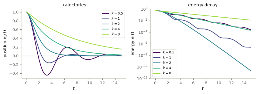
5. Control ↔︎ ML: two forward connections
- Feedback ↔︎ reinforcement learning. Reinforcement learning is “learning based on feedback”: there are no correct input–output pairs, but there is a reward. The common idea is that an action depends on the observed state. The difference is that a feedback law is designed from a known model, while in reinforcement learning a policy is learned from rewards.
- Damping ↔︎ momentum methods. The “heavy ball” picture of momentum in gradient descent is a damped second-order dynamics. Its damping parameter can be too small, giving oscillations, or too large, giving slow creeping, exactly as in the decay-rate figure above.
Key takeaways
- A control problem consists of a state equation, a set of admissible controls and an objective.
- Controllability: can the target be reached? Optimal control: which admissible control is best? Stabilization: is there a rule \(u=F(x)\) that makes the equilibrium asymptotically stable (stable and attracting), here for every initial state?
- Open loop: \(u=u(t)\), computed in advance. Closed loop: \(u=F(x(t))\), computed in real time from the state, so it can correct for unknown disturbances.
- Viscous damping is the feedback \(u=-kx_2\), and it makes the energy non-increasing: \(e'=-k(x_1')^2\).
- The decay rate is \(r(k)=k/2\) for \(k\le2\) and \(2/(k+\sqrt{k^2-4})\) for \(k\ge2\): it is maximal at critical damping, \(k=2\), and tends to \(0\) as \(k\to\infty\).
6. Exercises
★ conceptual · ★★ mathematical · ★★★ computational
- Which question is it? ★ Classify each problem as controllability, optimal control or stabilization, and say what the unknown is: (a) keep an inverted pendulum upright despite small pushes; (b) bring a crane load from rest at one point to rest at another point in exactly 20 s; (c) among all ways of doing (b), find the one using the least energy; (d) cruise control keeps a car at 100 km/h on hills.
- The oscillator. ★★ (a) Verify that \(x_1(t)=(1+t)e^{-t}\) solves \(x_1''+2x_1'+x_1=0\) with \(x_1(0)=1\), \(x_1'(0)=0\). (b) For \(k>2\), show that \(r(k)=2/(k+\sqrt{k^2-4})\) is strictly decreasing, and that \(k\,r(k)\to1\) as \(k\to\infty\). (c) For \(k>2\) and \(x^0=(1,0)\), write the solution as \(c_+e^{\lambda_+t}+c_-e^{\lambda_-t}\) and show that both coefficients are nonzero, so that the slow rate is actually observed.
- Open loop versus feedback. ★★ Consider the thermostat model \(x'=-x+u+d\) for a temperature deviation \(x\), with setpoint \(1\) and an unknown constant disturbance \(d\). (a) compute the limit of \(x(t)\) for the open-loop control \(u\equiv1\) and for the feedback \(u=1+L(1-x)\), for a constant unknown \(d\); (b) show that the feedback error tends to \(0\) as \(L\to\infty\); (c) now assume that the measurement is wrong by a constant bias \(\beta\), so the feedback uses \(x+\beta\) instead of \(x\). What is the limit, and what does a large \(L\) do to the effect of \(\beta\)?
- Energy is not enough. ★★ For \(x_1''+kx_1'+x_1=0\) we showed \(e'=-k(x_1')^2\le0\). (a) Does this inequality alone prove that \(e(t)\to0\)? Find the weak point. (b) Use the characteristic roots to prove that \(e(t)\to0\) exponentially for every \(k>0\).
- A stiffer spring. ★★★ Consider \(x_1''+kx_1'+\omega^2x_1=0\) with \(\omega>0\). Modify the decay-rate code of §4 to compute \(r(k;\omega)\) numerically for \(\omega\in\{0.5,1,2\}\) and \(0<k\le10\). Find the best damping \(k^*(\omega)\) and the best rate, and conjecture formulas. Then prove them from the characteristic roots.
# TODO: student exercise (Exercise 5)
# Build A = [[0, 1], [-omega**2, -k]] and compute the decay rate -max Re(eig(A)) on a grid of k,
# for omega in [0.5, 1, 2]. Plot the rates against k and locate the maximum.

def decay_rate(k, omega):
    ...  # your code here
    return None
Where are we going?
We have three questions and one example. Notebook 02 takes the first question, controllability, for linear systems \(x'=Ax+Bu\). It asks when a few controls can steer a system between arbitrary states, and it answers with the Kalman rank condition and an explicit steering control.
References
- J. C. Maxwell, On governors, Proceedings of the Royal Society of London 16 (1868), 270–283.
- N. Wiener, Cybernetics: or Control and Communication in the Animal and the Machine, MIT Press, 1948.
- R. Bellman, The theory of dynamic programming, Bulletin of the AMS 60 (1954), 503–515.
- L. S. Pontryagin, V. G. Boltyanskii, R. V. Gamkrelidze, E. F. Mishchenko, The Mathematical Theory of Optimal Processes, Interscience, 1962.
- R. E. Kalman, Contributions to the theory of optimal control, Boletín de la Sociedad Matemática Mexicana 5 (1960), 102–119.
- E. D. Sontag, Mathematical Control Theory: Deterministic Finite Dimensional Systems, 2nd ed., Springer, 1998.
- K. J. Åström, R. M. Murray, Feedback Systems: An Introduction for Scientists and Engineers, 2nd ed., Princeton University Press, 2021.