%matplotlib inline
import numpy as np
import torch
import matplotlib.pyplot as plt
from scipy.linalg import expm
from scipy.optimize import linear_sum_assignment
import plotting as P           # the course palette, the house style, and the figure helpers

torch.manual_seed(0)
# Independent streams, fixed in the protocol: data (transport atoms, then the initial conditions of Laboratory B),
# features (SA-NODE inner parameters), dev (exercises and reference levels), eval (final evaluation data,
# drawn once, after every choice is fixed).
rng_data, rng_features = np.random.default_rng(1601), np.random.default_rng(1602)
rng_dev, rng_eval = np.random.default_rng(1603), np.random.default_rng(1604);16 — Neural Transport and Learning Dynamics from Data
Mathematical Foundations of Control and Machine Learning — Winter 2026
Central question. How does a neural ODE move a probability distribution, how do we measure how well it does so, and can the same fields learn an unknown dynamics from trajectories?
A neural ODE moves points. When the points are many, samples of a distribution, it is natural to follow the distribution itself. A neural ODE then transports a probability measure, as generative “normalizing flows” do: neural transport. The same fields serve a second purpose, learning an unknown dynamics from trajectories. This notebook treats both, with two laboratories — A (transport) and B (learning) — and a protocol fixed before any evaluation data were drawn.
Table of Contents
- Transporting a measure — push-forward and the transport equation
- Measuring transport — the Wasserstein-1 distance
- Atoms to atoms, exactly
- Laws are not atoms — the neural transport theorem, and Laboratory A
- Learning a dynamics from trajectories — semi-autonomous neural ODEs, and Laboratory B
- Control ↔︎ ML
- From field errors to trajectory errors: Gronwall
- Numerical results and open directions
- Exercises
Notation. Densities and measures \(\rho\), \(\rho_0\), \(\rho_T\); velocity field \(V(x,t)\); Wasserstein-1 distance \(W_1\); \(\mathcal P^{ac}_c(\mathbb R^d)\) the compactly supported, absolutely continuous probability measures. The width is \(P\), and \(L\) counts switches.
Where are we?
Recap. One ReLU neuron with constant control freezes a half-space and moves the other exactly; shears move points along one direction without changing their “heights” (notebook 14). Monge’s problem between two samples is a linear program whose optimal plans are permutations.
The example throughout is the Gaussian-to-uniform transport: an initial law \(\rho_0=\mathcal N\big((0.5,0.5),\,0.15^2I\big)\) and a target law \(\rho_T=U([0,1]^2)\), represented by samples.
1. Transporting a measure: push-forward and the transport equation
The neural ODE \(x'=w(t)\sigma(a(t)\cdot x+b(t))\), \(x(0)=x_0\), defines a flow map \(\Phi_T:x_0\mapsto x(T)\). Its trajectories are the characteristics of the transport equation \[ \partial_t\rho+\operatorname{div}_x\big(V(x,t)\,\rho\big)=0,\qquad\rho(0)=\rho_0,\qquad V(x,t)=w(t)\sigma(a(t)\cdot x+b(t)), \] where \(V\) is Lipschitz in space: true for the ReLU, with piecewise-constant controls. The solution is the push-forward \(\rho(T)=\Phi_{T\#}\rho_0\): the mass that \(\rho_0\) puts on a set \(B\) is the mass that \(\rho(T)\) puts on \(\Phi_T(B)\). Equivalently, for every bounded continuous test function \(\varphi\), \[ \int\varphi\,d\rho(T)=\int\varphi\big(\Phi_T(x)\big)\,d\rho_0(x)\qquad\text{(the weak identity).} \] Two cases look different but follow the same rule.
- Atoms. If \(\rho_0=\sum_im_i\delta_{x_i}\), then \(\rho(T)=\sum_im_i\delta_{\Phi_T(x_i)}\). Each atom moves along its characteristic with its mass \(m_i\); no volume factor appears. Transporting an empirical measure means moving its points and keeping their weights.
- Densities. If \(\rho_0\) has a density and \(\Phi_T\) is a smooth bijection, the density at \(\Phi_T(x)\) is \(\rho_0(x)/|\det D\Phi_T(x)|\). Where the flow expands volume, the density drops. For one ReLU expansion action (\(w\parallel a\), \(a\cdot w>0\)), \(\det D\Phi_t=e^{(a\cdot w)t}\) on the active side and \(1\) on the frozen side.
Mass is conserved in both cases, and it is the weights (for atoms) or the density times volume (for densities) that carry it. The cell checks the weak identity for a density pushed by \(\Phi(x)=2x+1\) on the line, and the bookkeeping of masses for three atoms.
Predict. The uniform density on \([0,1]\) is pushed by \(\Phi(x)=2x+1\). What is the new density? What happens to atoms of masses \(0.5,0.3,0.2\)?
def samples_gauss_uniform(generator, n):
    # n points of rho_0 = N((0.5, 0.5), 0.15^2 I) and n points of rho_T = U([0, 1]^2)
    X0 = 0.5 + 0.15 * generator.standard_normal((n, 2))
    X1 = generator.uniform(0, 1, size=(n, 2))
    return X0, X1

X0_atoms, X1_atoms = samples_gauss_uniform(rng_data, n=8)

# Push-forward on the line by Phi(x) = 2x + 1.
Phi_line = lambda x: 2 * x + 1
nodes, weights = np.polynomial.legendre.leggauss(40)
x01, w01 = 0.5 * (nodes + 1), 0.5 * weights                      # quadrature on [0, 1]
x13, w13 = 2 + nodes, weights                                    # quadrature on [1, 3]
for name, phi in (("cos", np.cos), ("x^2", lambda x: x**2)):
    lhs = np.sum(w13 * 0.5 * phi(x13))                           # phi against the pushed density 1/2 on [1, 3]
    rhs = np.sum(w01 * 1.0 * phi(Phi_line(x01)))                 # phi(Phi(x)) against the uniform density on [0, 1]
    print(f"weak identity with phi = {name}: {lhs:.12f} = {rhs:.12f}")
atoms, masses = np.array([0.0, 0.4, 1.0]), np.array([0.5, 0.3, 0.2])
print("atoms", atoms, "-> ", Phi_line(atoms), "; masses stay", masses, "; total", masses.sum(),
      "; the density 1 on [0, 1] becomes the density 1/2 on [1, 3]")
weak identity with phi = cos: -0.350175488374 = -0.350175488374
weak identity with phi = x^2: 4.333333333333 = 4.333333333333
atoms [0. 0.4 1. ] -> [1. 1.8 3. ] ; masses stay [0.5 0.3 0.2] ; total 1.0 ; the density 1 on [0, 1] becomes the density 1/2 on [1, 3]Reading the output (answer to the prediction). The pushed density is \(\frac12\) on \([1,3]\): the interval has doubled, so the density halves, and the weak identity holds to quadrature accuracy for both test functions. The atoms move to \(1\), \(1.8\), \(3\) and keep their masses \(0.5\), \(0.3\), \(0.2\). In an empirical measure, no point becomes “lighter” because the flow spreads the points apart.
2. Measuring transport: the Wasserstein-1 distance
Success is measured with the Wasserstein-1 distance, \[ W_1(\mu,\nu)=\min_{\pi}\int|x-y|\,d\pi(x,y), \] the cheapest total distance travelled when moving \(\mu\) onto \(\nu\), minimized over transport plans \(\pi\) with marginals \(\mu\) and \(\nu\). This is the Kantorovich formulation, over plans, of Monge’s problem, which looks instead for a map \(T\) pushing \(\mu\) onto \(\nu\); a plan may split the mass of a point, a map may not.
- On the line, \(W_1(\mu,\nu)=\int_{\mathbb R}|F_\mu-F_\nu|\,dx=\int_0^1|F_\mu^{-1}(s)-F_\nu^{-1}(s)|\,ds\), with \(F\) the cumulative distribution functions. For two samples of equal size \(n\) and weights \(1/n\), it is the mean distance between the sorted samples: matching by quantiles is optimal.
- Between two samples of equal size \(n\) with weights \(1/n\) in \(\mathbb R^d\), the plans form the polytope of doubly stochastic matrices divided by \(n\), whose extreme points are the permutation matrices divided by \(n\) (Birkhoff–von Neumann). A linear cost attains its minimum at an extreme point, so an optimal plan can be taken to be a permutation, a Monge map, and \(W_1=\min_s\frac1n\sum_i|x_i-y_{s(i)}|\): an assignment problem with Euclidean cost. The optimal mean squared cost is \(W_2^2\), and \(W_2\) is its square root; the transport theorem of §4 uses \(W_1\), and we do not replace it by a sliced or squared surrogate.
The cell checks both computations on cases that can be done by hand.
def w1_1d(x, y, wx=None, wy=None):
    # W1 on the line: integral of |F_mu - F_nu| over the merged support
    x, y = np.asarray(x, float), np.asarray(y, float)
    wx = np.full(len(x), 1 / len(x)) if wx is None else np.asarray(wx, float)
    wy = np.full(len(y), 1 / len(y)) if wy is None else np.asarray(wy, float)
    grid = np.sort(np.concatenate([x, y]))
    F = lambda pts, w, t: np.sum(w[None, :] * (pts[None, :] <= t[:, None]), axis=1)
    mid = grid[:-1]
    return float(np.sum(np.abs(F(x, wx, mid) - F(y, wy, mid)) * np.diff(grid)))

def w1_assignment(X, Y):
    # W1 between equal-size samples with uniform weights: assignment with Euclidean cost
    cost = np.linalg.norm(X[:, None, :] - Y[None, :, :], axis=2)
    rows, cols = linear_sum_assignment(cost)
    return float(cost[rows, cols].mean()), cols

print("W1(delta_0, delta_1) =", w1_1d([0.0], [1.0]))
print("W1((delta_0 + delta_1)/2, delta_1/2) =", w1_1d([0.0, 1.0], [0.5]))
print("W1(0.25 delta_0 + 0.75 delta_1, delta_1) =", w1_1d([0.0, 1.0], [1.0], wx=[0.25, 0.75]),
      " (weights are masses)")
x_s, y_s = np.array([0.3, -1.0, 2.0, 0.7]), np.array([1.5, 0.0, -0.2, 0.4])
print(f"four points each: by CDFs {w1_1d(x_s, y_s):.6f}, "
      f"by sorted pairs {np.mean(np.abs(np.sort(x_s) - np.sort(y_s))):.6f}, "
      f"by assignment {w1_assignment(x_s[:, None], y_s[:, None])[0]:.6f}")
W1_atoms_before, match = w1_assignment(X0_atoms, X1_atoms)
print(f"atoms: W1 = {W1_atoms_before:.4f}, optimal assignment {match}")
W1(delta_0, delta_1) = 1.0
W1((delta_0 + delta_1)/2, delta_1/2) = 0.5
W1(0.25 delta_0 + 0.75 delta_1, delta_1) = 0.25 (weights are masses)
four points each: by CDFs 0.475000, by sorted pairs 0.475000, by assignment 0.475000
atoms: W1 = 0.3700, optimal assignment [4 1 2 6 7 3 0 5]3. Atoms to atoms, exactly
Atomic initial data can be driven to atomic final targets. In the plane, shears do it in two phases, following the two steps used for simultaneous control (control \(d-1\) coordinates, then the remaining coordinate):
- Phase 1: shears along \(e_1\), with heights \(x^{(2)}\), set every first coordinate to its target; second coordinates do not change.
- Phase 2: shears along \(e_2\), with heights \(x^{(1)}\) (now the target first coordinates), set every second coordinate to its target; first coordinates do not change.
Each phase is a triangular construction (sort the atoms by height, place one knot below each, and solve a lower-triangular system for the speeds), so each atom lands exactly on its target, given distinct initial second coordinates and distinct target first coordinates. Which atom goes to which target is a free choice. We take the optimal assignment for \(W_1\) computed above: theory of optimal transport → neural transport. The control is transport (i) of Laboratory A.
Predict. After transport (i), what is \(W_1\) between the transported atoms and the target atoms? How large must the controls be?
relu = lambda z: np.maximum(z, 0.0)

def shear_phase(X, required, a, u, T_phase):
    # the triangular shear construction: heights along a, motion along u (a.u = 0);
    # returns one layer (a, u, knot, coeff) per point, each of duration T_phase / n
    h = X @ a
    order = np.argsort(h)
    hs, req = h[order], required[order]
    knots = np.concatenate([[hs[0] - 1.0], 0.5 * (hs[:-1] + hs[1:])])
    coeffs = np.zeros(len(hs))
    for i in range(len(hs)):
        coeffs[i] = (req[i] - np.sum(coeffs[:i] * relu(hs[i] - knots[:i]))) / (hs[i] - knots[i])
    tau = T_phase / len(hs)
    return [(a.copy(), u.copy(), knots[i], coeffs[i], tau) for i in range(len(hs))]

def two_phase_transport(X0, targets, T=1.0):
    e1, e2 = np.eye(2)
    layers = shear_phase(X0, targets[:, 0] - X0[:, 0], a=e2, u=e1, T_phase=T / 2)
    X_mid = transport(X0, layers)
    return layers + shear_phase(X_mid, targets[:, 1] - X_mid[:, 1], a=e1, u=e2, T_phase=T / 2)

def transport(X, layers):
    # exact flow map of the shear layers (each is a parallel action: heights along a never change)
    Z = X.copy()
    for a, u, knot, coeff, tau in layers:
        Z = Z + np.outer(coeff * relu(Z @ a - knot), u)
    return Z

targets = X1_atoms[match]                                        # the optimal assignment for W1
layers_i = two_phase_transport(X0_atoms, targets, T=1.0)         # transport (i): 16 shear layers, width 1
path_atoms = [X0_atoms]
for layer in layers_i:
    path_atoms.append(transport(path_atoms[-1], [layer]))
atoms_after_i = path_atoms[-1]
print(f"layers {len(layers_i)} (switches {len(layers_i) - 1}); "
      f"largest speed {max(abs(L[3]) / L[4] for L in layers_i):.2e}")
print(f"max |transported atom - target| = {np.abs(atoms_after_i - targets).max():.1e};  "
      f"W1(transported atoms, target atoms) = {w1_assignment(atoms_after_i, X1_atoms)[0]:.1e}")

path = np.array(path_atoms)
fig, (ax1, ax2) = P.panels(2, figsize=(11, 4.1))
for i in range(len(X0_atoms)):
    ax1.annotate("", xy=targets[i], xytext=X0_atoms[i],
                 arrowprops=dict(arrowstyle="->", color=P.GREY, lw=0.8))
ax1.plot(*X0_atoms.T, "o", color=P.BLUE, label=r"atoms of $\rho_0$ (Gaussian)")
ax1.plot(*X1_atoms.T, "s", mfc="none", ms=9, color=P.ORANGE, label=r"atoms of $\rho_T$ (uniform)")
ax1.plot(*atoms_after_i.T, ".", color=P.INK, label="after transport (i)")
P.label(ax1, equal=True, title="optimal assignment and exact landing",
        legend={"fontsize": 8.5, "loc": "lower left"})
ax2.semilogy(np.arange(len(path)), np.abs(path - 0.5).max(axis=(1, 2)), "o-", color=P.BLUE)
ax2.axvline(len(layers_i) / 2, color=P.RULE, lw=0.7, ls=":")
P.label(ax2, "after layer (dotted: end of phase 1)", r"$\max_i|x_i-(0.5,0.5)|_\infty$",
        title="how far the atoms travel in between")
plt.show()
layers 16 (switches 15); largest speed 5.69e+03
max |transported atom - target| = 5.6e-16; W1(transported atoms, target atoms) = 2.5e-16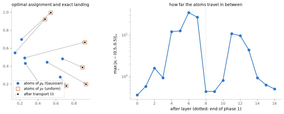
Figure 1. Transport (i) of the eight atoms. Left: the atoms of \(\rho_0\) (circles), of \(\rho_T\) (squares), the optimal \(W_1\) assignment (arrows) and the positions after the 16 shear layers (black dots). Right: the largest distance of an atom from the centre of the square after each layer, on a logarithmic scale.
Interpretation (answer to the prediction). Every atom lands on its target to rounding (printed), so \(W_1\) between the transported and target atoms is \(0\) up to rounding. The control is not small: the printed speeds are large, and the atoms make large excursions between the layers (right) before the last layers bring them back. Atoms can indeed be driven to atoms; the question of §4 is what this does to the distribution the atoms were drawn from.
4. Laws are not atoms
Theorem (Álvarez-López, Hadj Slimane and Zuazua, 2024), transcribed without its switch formula. Let \(d\ge1\), \(\rho_0\in\mathcal P^{ac}_c(\mathbb R^d)\) and \(\rho_T=U([0,1]^d)\). For any \(T>0\) and \(\varepsilon>0\), and width \(p\ge1\), there is a piecewise-constant control \((w,a,b)\in L^\infty\big((0,T);\mathbb R^{d\times p}\times\mathbb R^{p\times d}\times\mathbb R^p\big)\) such that the neural transport solution satisfies \(W_1(\rho(T),\rho_T)<\varepsilon\), with a finite number \(L\) of switches depending on \(d\), \(p\) and \(\varepsilon\). The proof: compress \(\rho_0\) into \([0,1]^d\); partition the cube into rectangles \(C_{i,j}\) and \(G_{i,j}\) carrying the same small masses under \(\rho_0\) and \(\rho_T\); transform each \(C_{i,j}\) into \(G_{i,j}\) by compressions and expansions.
Audit of the switch count. An explicit count \(L=\lceil2d/p\rceil+\big\lceil\frac{1}{p-d+1}\big(\frac{3^{1+d}\sqrt d}{\varepsilon}\big)^d\big\rceil-1\) has been stated for this construction, under the assumptions \(q\in[1,\frac d{d-1})\) and \(p\ge1\). As stated it cannot be checked: - the factor \(\frac1{p-d+1}\) is undefined for \(p=d-1\) and negative for \(p<d-1\), although \(p\ge1\) is allowed; - the parameter \(q\) appears in the hypotheses but nowhere in the conclusion; - the interval \([1,\frac d{d-1})\) is undefined for \(d=1\). We therefore do not reproduce the formula. What survives is qualitative: finitely many switches, growing as \(\varepsilon\to0\), with the factor \(\varepsilon^{-d}\) inside the expression suggesting a curse of dimension.
Hypotheses that matter here. The theorem concerns an absolutely continuous, compactly supported initial law, approximated in \(W_1\). The atoms of §3 are a different object, and exact landing of eight atoms says nothing about a law. Also, the Gaussian \(\rho_0\) of our example is not compactly supported, so the theorem does not apply to it as stated, although more than \(99.8\%\) of its mass lies in the unit square.
Laboratory A: two transports, judged on new samples. Both are fixed in the protocol before any evaluation sample was drawn. Every particle is moved by the same declared field, applied exactly.
- Transport (i): the exact atomic matching of §3.
- Transport (ii): compress/expand at the level of the law.
- Four expansions about the centre \((0.5,0.5)\). In each half-plane \(\{x^{(1)}>0.5\}\), \(\{x^{(1)}<0.5\}\), \(\{x^{(2)}>0.5\}\), \(\{x^{(2)}<0.5\}\) an action with \(w\parallel a\) and \(a\cdot w=\ln2\) acts for unit time, multiplying distances from the centre lines by \(2\). The factor is the ratio of standard deviations, \((1/\sqrt{12})/0.15\approx1.9\), rounded.
- Four contractions towards the sides of the unit square (\(a\cdot w=-3\)), which pull outlying points towards the square without letting them cross.
- These are the parallel, contraction and expansion actions of one ReLU neuron, the building blocks of the theorem’s proof, used here without any attempt at the full construction.
- Evaluation: 400 new points of \(\rho_0\) and 400 of \(\rho_T\), from the reserved stream, drawn after both transports were fixed. We report \(W_1\) before and after each transport, for the atoms and for the new samples.
Predict. Which transport will bring the new sample of \(\rho_0\) closer to the new sample of \(\rho_T\)?
def relu_action_exact(X, w, a, b, t):
    # closed-form solution of x' = w relu(a.x + b) with constant control
    s0 = X @ a + b
    c = a @ w
    factor = (np.expm1(c * t) / c) if abs(c) > 1e-14 else t
    return X + np.outer(relu(s0) * factor, w)

e1, e2 = np.eye(2)
c_exp, c_con = np.log(2.0), 3.0
actions_ii = [(c_exp * e1, e1, -0.5), (-c_exp * e1, -e1, 0.5),
              (c_exp * e2, e2, -0.5), (-c_exp * e2, -e2, 0.5),      # expansions about the centre lines
              (-c_con * e1, e1, -1.0), (c_con * e1, -e1, 0.0),
              (-c_con * e2, e2, -1.0), (c_con * e2, -e2, 0.0)]      # contractions towards the sides

def transport_ii(X):
    for w, a, b in actions_ii:                   # each action: x' = w max(a.x + b, 0) for unit time, exact
        X = relu_action_exact(X, w, a, b, 1.0)
    return X

# Final evaluation of Laboratory A: new samples, drawn once, after both transports were fixed.
X0_eval, X1_eval = samples_gauss_uniform(rng_eval, n=400)
labA = {"before": {"atoms": W1_atoms_before, "new samples": w1_assignment(X0_eval, X1_eval)[0]},
        "(i) atomic matching": {"atoms": w1_assignment(transport(X0_atoms, layers_i), X1_atoms)[0],
                                "new samples": w1_assignment(transport(X0_eval, layers_i), X1_eval)[0]},
        "(ii) compress/expand": {"atoms": w1_assignment(transport_ii(X0_atoms), X1_atoms)[0],
                                 "new samples": w1_assignment(transport_ii(X0_eval), X1_eval)[0]}}
print("                          W1 atoms (n = 8)    W1 new samples (n = 400)")
for name, r in labA.items():
    print(f"{name:24s}  {r['atoms']:16.2e}    {r['new samples']:22.4f}")
# Reference level (development stream, not evaluation data): W1 between two independent samples of rho_T.
W1_reference = w1_assignment(samples_gauss_uniform(rng_dev, n=400)[1], samples_gauss_uniform(rng_dev, n=400)[1])[0]
print(f"reference: W1 between two independent samples of U([0,1]^2), n = 400 each: {W1_reference:.4f}")
sample_i, sample_ii = transport(X0_eval, layers_i), transport_ii(X0_eval)
print(f"after (i), largest |x| of the transported sample {np.abs(sample_i).max():.1e}; after (ii), fraction outside "
      f"[0,1]^2 {np.mean(np.any((sample_ii < 0) | (sample_ii > 1), axis=1)):.3f} "
      f"(contractions approach the sides, never cross)")

fig, (ax1, ax2) = P.panels(2, figsize=(11, 4.3))
ax1.plot(*sample_i.T, ".", ms=3, color=P.BLUE, label="new sample of $\\rho_0$ after (i)")
ax1.plot(*X1_eval.T, ".", ms=3, color=P.ORANGE, label="new sample of $\\rho_T$")
ax1.set_xscale("symlog", linthresh=1); ax1.set_yscale("symlog", linthresh=1)
P.label(ax1, title="(i) atomic matching: symmetric log axes")
ax2.plot(*sample_ii.T, ".", ms=3, color=P.BLUE, label="new sample of $\\rho_0$ after (ii)")
ax2.plot(*X1_eval.T, ".", ms=3, color=P.ORANGE, label="new sample of $\\rho_T$")
ax2.plot([0, 1, 1, 0, 0], [0, 0, 1, 1, 0], color=P.INK, lw=0.8)
P.label(ax2, equal=True, title="(ii) compress/expand",
        legend={"fontsize": 8.5, "loc": "upper center", "bbox_to_anchor": (0.5, -0.08), "ncol": 2})
plt.show()
W1 atoms (n = 8) W1 new samples (n = 400)
before 3.70e-01 0.2106
(i) atomic matching 2.50e-16 165.8772
(ii) compress/expand 4.00e-01 0.0808
reference: W1 between two independent samples of U([0,1]^2), n = 400 each: 0.0518
after (i), largest |x| of the transported sample 3.6e+03; after (ii), fraction outside [0,1]^2 0.168 (contractions approach the sides, never cross)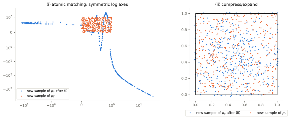
Figure 2. Laboratory A on the evaluation samples. Left: 400 new points of \(\rho_0\) after transport (i) (symmetric logarithmic axes) and 400 new points of \(\rho_T\). Right: the same new points of \(\rho_0\) after transport (ii), the new points of \(\rho_T\), and the unit square.
Interpretation (answer to the prediction). Transport (ii). Transport (i) is exact on the eight atoms, but it sends the new sample of \(\rho_0\) far away (printed \(W_1\) values and largest \(|x|\)): its speeds were chosen to land eight points, and every other point is moved by the same piecewise-linear displacements, which are enormous between the atoms. Transport (ii) never looks at the atoms: their \(W_1\) barely changes. It brings the new samples much closer, because the expansions spread the Gaussian mass over the square and the contractions pull the tails back towards its sides; a fraction of the points stays just outside, since a contraction never crosses its hyperplane. For scale, two independent samples of the uniform law of the same size are already at a printed reference distance from each other: \(W_1\) between finite samples includes sampling fluctuation. Neither transport is the construction of the theorem. The comparison shows that a transport must be judged on the law, with new samples, and that exact matching of a sample is the transport analogue of interpolating training data.
5. Learning a dynamics from trajectories: semi-autonomous neural ODEs
The model. A semi-autonomous neural ODE (SA-NODE; Li, Liu, Liverani and Zuazua, 2026) is \[ x'(t)=\sum_{i=1}^Pw_i\,\sigma\big(a_i^1\cdot x(t)+a_i^2\,t+b_i\big),\qquad w_i\in\mathbb R^d,\ a_i^1\in\mathbb R^d,\ a_i^2\in\mathbb R,\ b_i\in\mathbb R . \] The parameters do not depend on time; time enters as an extra input. Compared with a neural ODE whose controls change with \(t\), this greatly reduces the complexity of the model. In matrix form, \(x'=W\sigma(A_1x+a_2t+b)\) with \(W\in\mathbb R^{d\times P}\), \(A_1\in\mathbb R^{P\times d}\), \(a_2,b\in\mathbb R^P\).
Reported results (transcribed, not proved here). - Approximation of trajectories. If the true field \(f(z,t)\) is uniformly Lipschitz in \(z\) with respect to \(t\), then for every compact \(K\) and \(\varepsilon>0\) there is \(\bar p\) such that for every \(P\ge\bar p\) some parameters give \(\|z_{z_0}-x_{z_0}\|_{L^\infty(0,T)}\le\varepsilon\) for all initial data \(z_0\in K\). Proof: apply the universal approximation property to \(f\), then Gronwall estimates. - A rate. If \(f\in H^k_{\rm loc}\) with \(k>\frac{d+1}2+2\), then \(\sup_t\int_K|z_{z_0}(t)-x_{z_0}(t)|^2dz_0\le C_{T,K,f}/P\). - Transport. For a probability measure \(\rho_0\) supported in a compact \(K\) with \(\rho_0\in L^2(K)\), \(\sup_tW_1(\rho(t),\rho_\Theta(t))\le C_{T,f,\rho_0}/\sqrt P\).
A self-contained setting in which the first argument works (our sufficient hypotheses). Let \(f\) be continuous on \(\mathbb R^d\times[0,T]\) and globally Lipschitz in \(z\), uniformly in \(t\). Then every solution exists on \([0,T]\), and the trajectories from \(K\) stay in a compact tube \(K_T\). Approximate \(f\) uniformly on a compact neighbourhood of \(K_T\) by a ReLU field (universal approximation), so that the model trajectories also stay there for a small enough error. Gronwall’s inequality (§7) then gives the uniform bound. For the rate, local Sobolev regularity alone does not even guarantee that trajectories exist up to time \(T\): \(x'=x^2\) is smooth and its solutions explode in finite time. One must also assume that the trajectories considered exist on \([0,T]\) and remain in a controlled domain, for instance under the global Lipschitz hypothesis. The transport rate inherits the hypotheses on the field used for the trajectory rate, together with a probability density in \(L^2\) with compact support; it is not a statement for arbitrary fields.
The last two rates are not interchangeable. \(C/P\) bounds an integrated squared trajectory error, so the root-mean-square error is of order \(1/\sqrt P\). \(C/\sqrt P\) bounds a \(W_1\) distance between densities. Both are existence statements about some parameters, not about the parameters our fitting procedure returns (§7).
Laboratory B. The dynamics to learn is \[
z_1'=z_2,\qquad z_2'=-2z_1-3z_2,
\] the harmonic oscillator \(x_1''+x_1=u\) under the feedback \(u=-x_1-3x_2\). The protocol fixes everything below before the evaluation data exist. - Trajectories: on \([0,3]\), 31 sampling times, computed exactly by the matrix exponential, from initial conditions uniform on \([-1,1]^2\). 20 trajectories are for training and 10 for validation. The split is by whole trajectories, so no trajectory contributes to two sets. - Privileged derivative targets. The fit uses the true field \(f(z)\) at the training points. Raw trajectory data would not provide it; it would have to be estimated, for instance by finite differences. We declare this simplification. - Training only the outer weights (a simplification). The inner parameters \((A_1,a_2,b)\) are drawn once, at random, from the stream features; a model of width \(P\) uses the first \(P\) neurons. \(W\) is fitted by ridge least squares, minimizing \(\frac1M\sum_j|W\Phi_j-f_j|^2+\lambda|W|_F^2\). No gradient is needed, since the inner parameters are not trained. - Choice on validation data: \(P\in\{10,20,40,80,160,320\}\) and \(\lambda\in\{10^{-8},10^{-6},10^{-4},10^{-2}\}\) are chosen by the mean, over validation trajectories, of the trajectory error, the largest distance between the true and the model trajectory over the sampling times. Each model trajectory is a rollout of the fitted SA-NODE from the true initial condition. - One final evaluation, for the chosen model only, on new initial conditions from the reserved stream, in two strata declared in advance: 20 in the training region \([-1,1]^2\), and 20 outside it (in \([-2,2]^2\) with \(\|z_0\|_\infty>1\)).
Predict. Will the model that fits the field best on the training points also have the smallest trajectory errors on validation? And how will the errors outside the training region compare?
A_cl = np.array([[0.0, 1.0], [-2.0, -3.0]])                      # z1' = z2, z2' = -2 z1 - 3 z2
t_grid = np.linspace(0.0, 3.0, 31)
exact_trajectory = lambda z0: np.array([expm(A_cl * t) @ z0 for t in t_grid])
ic_train = rng_data.uniform(-1, 1, size=(20, 2))
ic_val = rng_data.uniform(-1, 1, size=(10, 2))
Z_train = np.array([exact_trajectory(z0) for z0 in ic_train])
Z_val = np.array([exact_trajectory(z0) for z0 in ic_val])
P_max = 320
A1_all = rng_features.normal(size=(P_max, 2))
a2_all = rng_features.normal(size=P_max)
b_all = rng_features.uniform(-1, 1, size=P_max)
Z_pts, t_pts = Z_train.reshape(-1, 2), np.tile(t_grid, len(ic_train))
F_pts = Z_pts @ A_cl.T                                           # privileged derivative targets f(z) = A_cl z
widths, lams = [10, 20, 40, 80, 160, 320], [1e-8, 1e-6, 1e-4, 1e-2]

def sa_features(Z, t, A1, a2, b):
    return relu(Z @ A1.T + np.outer(np.atleast_1d(t), a2) + b)   # (M, P)

def fit_outer_weights(Phi, F, lam):
    M = len(F)
    return np.linalg.solve(Phi.T @ Phi / M + lam * np.eye(Phi.shape[1]), Phi.T @ F / M).T

def sa_node_rollout(z0, W, A1, a2, b, ts, substeps=2):
    # RK4 on the grid: x' = W sigma(A1 x + a2 t + b)
    f = lambda t, x: W @ relu(A1 @ x + a2 * t + b)
    xs = [np.asarray(z0, float)]
    for t0, t1 in zip(ts[:-1], ts[1:]):
        x, h = xs[-1], (t1 - t0) / substeps
        for s in range(substeps):
            t = t0 + s * h
            k1 = f(t, x); k2 = f(t + h / 2, x + h / 2 * k1)
            k3 = f(t + h / 2, x + h / 2 * k2); k4 = f(t + h, x + h * k3)
            x = x + h / 6 * (k1 + 2 * k2 + 2 * k3 + k4)
        xs.append(x)
    return np.array(xs)

trajectory_error = lambda Z_true, X_model: float(np.linalg.norm(Z_true - X_model, axis=1).max())

def fit_sa_node(Pw, lam):
    inner = (A1_all[:Pw], a2_all[:Pw], b_all[:Pw])
    Phi = sa_features(Z_pts, t_pts, *inner)
    W = fit_outer_weights(Phi, F_pts, lam)
    return W, inner, float(np.sqrt(np.mean(np.sum((Phi @ W.T - F_pts) ** 2, axis=1))))

def trajectory_errors(W, inner, ics, Z_true):
    return np.array([trajectory_error(Z, sa_node_rollout(z0, W, *inner, t_grid)) for z0, Z in zip(ics, Z_true)])

table_B, models_B = {}, {}
for Pw in widths:
    for lam in lams:
        W, inner, der = fit_sa_node(Pw, lam)
        err = trajectory_errors(W, inner, ic_val, Z_val)
        models_B[(Pw, lam)] = (W, inner)
        table_B[(Pw, lam)] = {"train rmse": der, "val mean": float(err.mean()), "val max": float(err.max())}
best_B = min(table_B, key=lambda k: (table_B[k]["val mean"], k[0], -k[1]))
print("   P     lambda   training derivative rmse   validation trajectory error: mean, max")
for (Pw, lam), r in table_B.items():
    print(f"{Pw:4d}   {lam:7.0e}   {r['train rmse']:24.2e}   {r['val mean']:10.2e}, {r['val max']:.2e}"
          + ("  <- chosen" if (Pw, lam) == best_B else ""))
best_field = min(table_B, key=lambda k: table_B[k]["train rmse"])
print(f"best training field fit: {best_field}, validation mean {table_B[best_field]['val mean']:.2e}")

fig, ax = P.panels(figsize=(7.2, 3.9))
for lam, col in zip(lams, (P.BLUE, P.AQUA, P.MAGENTA, P.ORANGE)):
    ax.loglog(widths, [table_B[(Pw, lam)]["val mean"] for Pw in widths], "o-", color=col,
              label=f"validation, $\\lambda$ = {lam:.0e}")
    ax.loglog(widths, [table_B[(Pw, lam)]["train rmse"] for Pw in widths], ":", color=col, lw=1)
ax.plot(best_B[0], table_B[best_B]["val mean"], "*", ms=14, color=P.INK, mfc="gold", label="chosen")
P.label(ax, "width $P$", "error", title="solid: validation trajectory error; dotted: training field error",
        legend={"fontsize": 8.5, "ncol": 2})
plt.show()
P lambda training derivative rmse validation trajectory error: mean, max
10 1e-08 1.74e-01 1.11e-01, 2.57e-01
10 1e-06 1.74e-01 1.11e-01, 2.57e-01
10 1e-04 1.74e-01 1.11e-01, 2.68e-01
10 1e-02 2.33e-01 1.68e-01, 4.44e-01
20 1e-08 9.06e-02 4.32e-02, 9.69e-02
20 1e-06 9.06e-02 4.32e-02, 9.69e-02
20 1e-04 9.30e-02 4.65e-02, 1.01e-01
20 1e-02 1.49e-01 9.75e-02, 3.09e-01
40 1e-08 1.53e-02 8.10e-03, 1.53e-02
40 1e-06 1.56e-02 8.20e-03, 1.84e-02
40 1e-04 2.24e-02 1.17e-02, 2.58e-02
40 1e-02 6.55e-02 3.52e-02, 1.17e-01
80 1e-08 3.12e-03 2.27e-03, 5.81e-03
80 1e-06 4.28e-03 3.27e-03, 6.65e-03
80 1e-04 1.02e-02 6.47e-03, 1.59e-02
80 1e-02 3.42e-02 1.32e-02, 3.89e-02
160 1e-08 5.98e-05 3.83e-04, 1.74e-03 <- chosen
160 1e-06 1.02e-03 1.70e-03, 3.19e-03
160 1e-04 4.25e-03 4.20e-03, 1.21e-02
160 1e-02 1.93e-02 6.84e-03, 1.15e-02
320 1e-08 3.14e-05 2.18e-03, 9.00e-03
320 1e-06 4.02e-04 2.11e-03, 6.64e-03
320 1e-04 2.13e-03 3.11e-03, 7.00e-03
320 1e-02 1.31e-02 5.19e-03, 1.01e-02
best training field fit: (320, 1e-08), validation mean 2.18e-03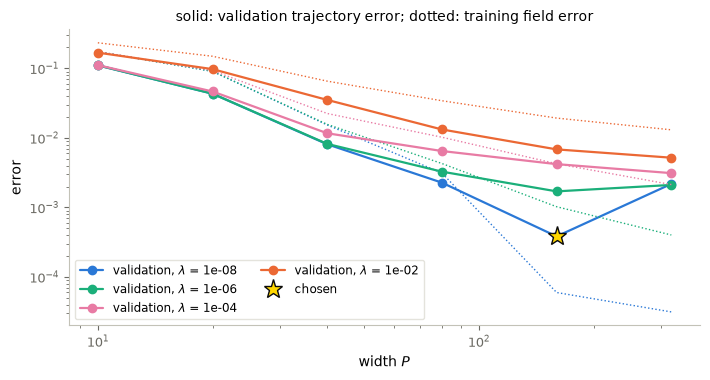
Figure 3. Laboratory B, choice on validation data. For each regularization \(\lambda\): the mean validation trajectory error (solid) and the root-mean-square field error on the training points (dotted), against the width \(P\). The star marks the model chosen.
Interpretation (answer to the first part of the prediction). No. Compare the printed table: the best field fit on the training points (the largest width at the smallest \(\lambda\)) is not the chosen model. The validation trajectory error improves with width only up to a point and then turns upward at the largest width, while the training field error keeps falling: fitting the field ever more precisely at the training points eventually stops helping, and then hurts, the trajectories elsewhere. The largest \(\lambda\) underfits at every width.
# Final evaluation of Laboratory B: new initial conditions from the reserved stream, drawn once,
# after the choice above; the chosen model only.
ic_in = rng_eval.uniform(-1, 1, size=(20, 2))
ic_out = []
while len(ic_out) < 20:
    z0 = rng_eval.uniform(-2, 2, size=2)
    if np.abs(z0).max() > 1:
        ic_out.append(z0)
ic_out = np.array(ic_out)
W_B, inner_B = models_B[best_B]
for name, ics in (("in the training region", ic_in), ("outside the training region", ic_out)):
    Z_true = np.array([exact_trajectory(z0) for z0 in ics])
    err = trajectory_errors(W_B, inner_B, ics, Z_true)
    print(f"{name:28s}: trajectory error mean {err.mean():.2e}, max {err.max():.2e}")

fig, axes = P.panels(2, figsize=(11, 4.1))
for ax, (name, ics) in zip(axes, (("in the training region", ic_in), ("outside the training region", ic_out))):
    for z0 in ics[:8]:
        Z = exact_trajectory(z0)
        X = sa_node_rollout(z0, W_B, *inner_B, t_grid)
        ax.plot(*Z.T, color=P.GREY, lw=2)
        ax.plot(*X.T, "--", color=P.BLUE, lw=1.2)
        ax.plot(*z0, "o", color=P.ORANGE, ms=4)
    ax.plot([-1, 1, 1, -1, -1], [-1, -1, 1, 1, -1], ":", color=P.INK, lw=0.8)
    P.label(ax, "$z_1$", "$z_2$", equal=True, title=f"{name}: true (grey) and SA-NODE (dashed)")
plt.show()
in the training region : trajectory error mean 3.76e-03, max 2.17e-02
outside the training region : trajectory error mean 1.18e-01, max 3.77e-01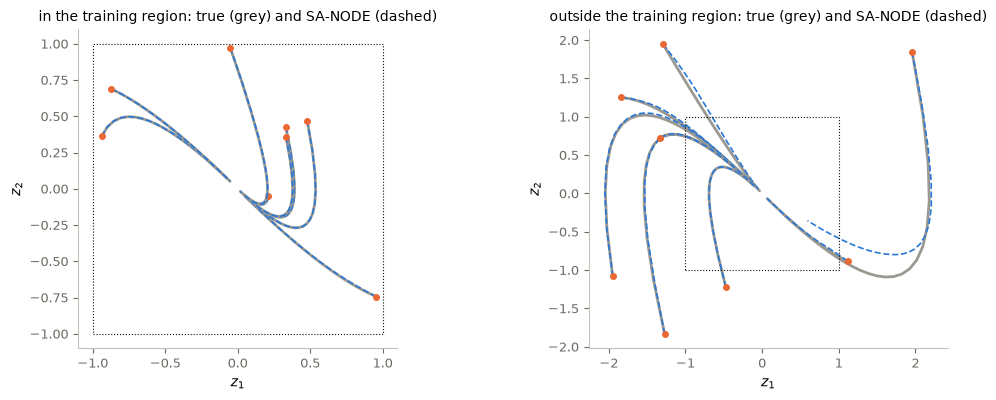
Figure 4. Laboratory B, final evaluation: eight of the twenty new trajectories of each stratum, true (grey) and rolled out by the chosen SA-NODE (dashed), with the training region \([-1,1]^2\) dotted.
Interpretation (answer to the second part of the prediction). In the training region the final errors (printed) are of the size seen on validation. Outside it they are markedly larger: those trajectories start where there were no training data, and the field error there is not controlled by the fit (§7). They still look qualitatively right because the true dynamics is stable and carries them into the training region, where the model is accurate. Both strata were declared before the data were drawn, and the numbers were computed once, after the choice.
6. Control ↔︎ ML
- Generative modelling = transport of measures by a controlled flow. DIRECT CONNECTION. Normalizing flows push a simple law to a target law; here the “control” is the neural field and the target is reached in \(W_1\).
- Optimal transport → neural transport. DIRECT CONNECTION. The optimal assignment chose which atom goes where in transport (i).
- Learning a dynamics = system identification. DIRECT CONNECTION. The SA-NODE is a model of an unknown vector field fitted to trajectories. Its error on new trajectories, not its fit to the field, is what matters, and Gronwall’s inequality links the two (§7).
- Atoms versus laws, fit versus generalization. MATHEMATICAL ANALOGY with interpolation and classification. Driving finitely many atoms exactly is the transport analogue of interpolating training data. It says nothing about the law, just as exact classification of training points said nothing about new points.
7. From field errors to trajectory errors: Gronwall
Let \(z'=f(z,t)\) be the true dynamics and \(x'=f_\Theta(x,t)\) the model, with the same initial value, and suppose \(f_\Theta\) is Lipschitz in \(x\) with constant \(L_\Theta\). Then, with \(\delta=\sup_{s\le t}|f(z(s),s)-f_\Theta(z(s),s)|\), the field error along the true trajectory, \[ |z(t)-x(t)|\le\int_0^t|f(z)-f_\Theta(z)|\,ds+\int_0^t|f_\Theta(z)-f_\Theta(x)|\,ds\le\delta t+L_\Theta\!\int_0^t|z-x|\,ds, \] and Gronwall’s lemma gives \(|z(t)-x(t)|\le\delta\,\frac{e^{L_\Theta t}-1}{L_\Theta}\) (and \(\le\delta t\) if \(L_\Theta=0\)). This is the second step of the approximation proofs of §5. It explains why a good field fit near the data is not enough. The error is amplified by \(e^{L_\Theta T}\), and \(\delta\) is the field error along the trajectory, which outside the training region is not controlled by the fit. For a ReLU field, \(L_\Theta\le\|W\|\,\|A_1\|\) (spectral norms). The cell evaluates the formula for the chosen model on the validation trajectories, as an estimate on the time grid. It replaces \(\delta\) by the largest field error over the 31 sampling times, which is not the supremum over \([0,T]\), and compares the result with the trajectory error, itself measured only at the sampling times. This shows the size of the formula; it does not verify the continuous inequality. Certifying it would need a bound on the field error between the grid points, for instance from a Lipschitz bound in time of the residual and the grid spacing. A finer grid alone would certify nothing either.
About the rates. The theorems guarantee that some parameters achieve errors of order \(1/\sqrt P\) (root-mean-square) or \(C/\sqrt P\) in \(W_1\). Our inner parameters are random and not optimized, and \(\lambda\) is chosen on validation data, so the curves of Figure 3 are not a test of those rates.
L_theta = np.linalg.norm(W_B, 2) * np.linalg.norm(inner_B[0], 2)
T_end = t_grid[-1]
factor = T_end if L_theta == 0 else np.expm1(L_theta * T_end) / L_theta    # (e^(LT) - 1)/L
rows = []
for z0, Z in zip(ic_val, Z_val):
    Phi_traj = sa_features(Z, t_grid, *inner_B)
    delta_grid = np.linalg.norm(Z @ A_cl.T - Phi_traj @ W_B.T, axis=1).max()    # max over the sampling times only
    observed = trajectory_error(Z, sa_node_rollout(z0, W_B, *inner_B, t_grid))  # also measured at the sampling times
    rows.append((delta_grid, observed, delta_grid * factor))
rows = np.array(rows)
print(f"L_Theta <= {L_theta:.2f};  factor (e^(L T) - 1)/L = {factor:.2e}")
print("grid field error, grid trajectory error, grid estimate of the Gronwall formula (not a certified bound):")
print(rows)
L_Theta <= 33.29; factor (e^(L T) - 1)/L = 7.19e+41
grid field error, grid trajectory error, grid estimate of the Gronwall formula (not a certified bound):
[[4.75196567e-04 2.51154798e-05 3.41640254e+38]
[4.59864296e-04 8.52639537e-05 3.30617193e+38]
[8.40824412e-04 6.68971958e-05 6.04506610e+38]
[1.29221842e-03 7.55878763e-05 9.29034135e+38]
[3.07064280e-03 5.50100436e-04 2.20762366e+39]
[1.13981291e-03 1.18746260e-04 8.19462936e+38]
[3.02136198e-03 4.26110874e-04 2.17219346e+39]
[2.62413921e-03 2.14891987e-04 1.88661209e+39]
[7.79594755e-02 1.73854144e-03 5.60485847e+40]
[2.97866194e-03 5.32425812e-04 2.14149447e+39]]Reading the output. The grid estimate of the formula exceeds the observed errors by many orders of magnitude: the printed factor \((e^{L_\Theta T}-1)/L_\Theta\) is astronomically large, while the observed errors are small. Both sides are evaluated on the time grid, so this comparison is an illustration of the size of the formula, not a verification of the inequality. Two reasons explain the gap. The product of norms vastly overestimates the Lipschitz constant that matters along the trajectories. And the true dynamics is asymptotically stable (eigenvalues \(-1\) and \(-2\)), which a worst-case estimate ignores. It is not a contraction in the Euclidean norm: the symmetric part of \(A_{\rm cl}\) has a positive eigenvalue. Gronwall’s inequality explains the mechanism: errors are driven by the field error along the trajectory and amplified by the flow. It does not predict their size.
8. Numerical results and open directions
- Pendulum: the same SA-NODE construction learns \(z_1'=z_2\), \(z_2'=-\sin z_1\) (Exercise 5).
- Transport of a density (ongoing work on optimal fluid mixing): SA-NODEs approximate the transport equation of Doswell frontogenesis, \(\partial_t\rho+\operatorname{div}\big(\rho\,(-yg(r),xg(r))\big)=0\), whose exact solution is known.
- Comparison with vanilla NODEs. On the linear system of Laboratory B and on a non-autonomous one, reported maximum trajectory errors are \(4.65\cdot10^{-2}\) to \(1.58\cdot10^{-2}\) for SA-NODEs with 1200–12000 degrees of freedom, against \(2.6\cdot10^{-1}\) to \(9.2\cdot10^{-2}\) for vanilla NODEs with 50000–500000 (autonomous case): better accuracy with fewer parameters. These numbers come from a different training procedure (all parameters trained) and are not comparable with ours.
- Statistical error. Chebyshev’s inequality allows estimating the statistical error of sampling for normalizing flows. The distance between an empirical sample and its law is itself a random quantity, which is why Laboratory A compares two samples and why its numbers have sampling fluctuation.
- Perspectives: momentum ResNets, width/depth trade-offs, dimensionality and probabilities, federated learning, relaxed neural ODEs; and, for digital twins, scalability, reliability and generalization.
Key takeaways
- A neural ODE transports a measure by push-forward; the trajectories are the characteristics of the transport equation. Atoms keep their masses; densities change by the volume factor.
- \(W_1\) is computed by quantiles in one dimension and, between equal-size samples, by an assignment with Euclidean cost.
- Finitely many atoms can be driven exactly to finitely many targets (two phases of shears in the plane), but that does not transport the law they were drawn from.
- The neural transport theorem concerns absolutely continuous, compactly supported laws approximated in \(W_1\); its printed switch count cannot be checked as stated.
- SA-NODEs with time-independent parameters can learn a dynamics; trajectories, not field values, must be split, validated and evaluated, and Gronwall’s inequality links field errors to trajectory errors.
9. Exercises
★ conceptual · ★★ mathematical · ★★★ computational
- Mass and volume. ★ One ReLU expansion action \(x'=w\sigma(a\cdot x+b)\) with \(w=c\,a\), \(|a|=1\), \(c>0\), acts for a time \(t\) on the plane. (a) Show that on the active side it maps \(x\) to \(x+a\,s(x)(e^{ct}-1)\), \(s=a\cdot x+b\), and compute its Jacobian determinant. (b) A density \(\rho_0\) is pushed forward: what is the new density at the image of a point of the active side? (c) An atom of mass \(0.3\) sits on the active side: what is its mass after the action?
- \(W_1\) on the line. ★★ Let \(\mu=\frac13(\delta_0+\delta_1+\delta_3)\) and \(\nu=\frac13(\delta_1+\delta_2+\delta_2)\). (a) Compute \(W_1(\mu,\nu)\) from \(\int|F_\mu-F_\nu|\) by hand. (b) Check that the sorted-pairs formula gives the same, and compare with
w1_1d. (c) Show by an example that matching the points in a non-monotone way can cost more. - Gronwall. ★★ (a) Prove Gronwall’s lemma in the form used in §7: if \(e(t)\le\delta t+L\int_0^te(s)\,ds\) with \(e\) continuous and non-negative, then \(e(t)\le\delta(e^{Lt}-1)/L\). (b) Why does the estimate use the field error along the true trajectory? Write the alternative estimate with the model trajectory and the Lipschitz constant of \(f\). (c) Evaluate the factor \((e^{LT}-1)/L\) for \(L=\|A_{\rm cl}\|\) and \(T=3\).
- Euclidean or squared cost? ★★ (a) Find two sets of three points in the plane whose optimal matching for the cost \(|x-y|\) differs from the optimal matching for \(|x-y|^2\), by a small search over configurations drawn from the stream
dev. (b) Which of the two would change the value reported in Laboratory A, and why does the transport theorem use \(W_1\)? - The pendulum. ★★★ Repeat Laboratory B for the pendulum \(z_1'=z_2\), \(z_2'=-\sin z_1\): exact trajectories are no longer available in closed form, so compute them with
solve_ivpat tight tolerance. Use the same features, grid and selection rule, and report validation errors only (the evaluation stream belongs to Laboratory B’s single final evaluation and must not be reused). - Width and validation error. ★★★ From the table of Laboratory B: (a) plot, for each \(P\), the best validation error over \(\lambda\), on log–log axes, together with reference lines \(\propto P^{-1}\) and \(\propto P^{-1/2}\). (b) Which slope do the data resemble, over which range of \(P\)? (c) Explain why this comparison cannot confirm or refute the reported rates.
# TODO: student exercise (Exercise 5)
# Return the pendulum field (z2, -sin z1) at every row of Z, shape (M, 2).

def pendulum_field(Z):
    ...  # your code here
    return None
Where are we going?
Networks have now been read as control systems: shallow networks as linear combinations of features, residual networks as discretized controlled ODEs trained by adjoints, classification as simultaneous control, attention as interacting particles, and generative modelling and system identification as transport and learning of flows. The recurring lesson is the distinction between what a control can achieve on given data and what a model predicts on new data, which only a protocol fixed in advance can measure.
Notebook 17 makes the transport stochastic: diffusion models reverse a noising flow, with the heat equation and score matching in the leading roles.
References
- D. Ruiz-Balet, E. Zuazua, Neural ODE control for classification, approximation, and transport, SIAM Review 65 (2023), 735–773.
- A. Álvarez-López, R. Hadj Slimane, E. Zuazua, Interplay between depth and width for interpolation in neural ODEs, Neural Networks 180 (2024), 106640.
- Z. Li, K. Liu, L. Liverani, E. Zuazua, Universal approximation of dynamical systems by semi-autonomous neural ODEs and applications, SIAM Journal on Numerical Analysis 64 (2026), 193–223.
- C. Villani, Optimal Transport: Old and New, Springer, 2009.
- G. Peyré, M. Cuturi, Computational optimal transport, Foundations and Trends in Machine Learning 11 (2019), 355–607.
- D. Rezende, S. Mohamed, Variational inference with normalizing flows, ICML 2015.