%matplotlib inline
import numpy as np
import torch
import matplotlib.pyplot as plt
import plotting as P           # the course palette, the house style, and the figure helpers

torch.manual_seed(0)
torch.set_default_dtype(torch.float64) # the duality checks below are run to ~1e-1003 — Observability, Duality and the Construction of Controls
Mathematical Foundations of Control and Machine Learning — Winter 2026
Central question. How can the problem of finding a control be transformed into an optimization problem for an adjoint system?
This notebook builds one chain, one justified step at a time: controllability → duality → adjoint system → observability → coercivity → minimization → control.
Table of Contents
- Why introduce an adjoint? — the adjoint appears by itself
- The adjoint system — backward in time, no control
- The fundamental duality identity — a conservation law with a source
- From the identity to a functional — reverse-engineering HUM
- Observability and coercivity — the four links of the chain
- Constructing the control — the main theorem
- Why is this the minimum-\(L^2\) control? — Pythagoras in \(L^2\)
- The Gramian interpretation — the Hessian of the dual functional
- Computational laboratory — the harmonic oscillator step by step; the near-uncontrollable family losing controllability
- Optimization preview — conditioning slows gradient descent
- What changes in infinite dimension? — the heat equation
- Control ↔︎ ML connection — adjoints and backpropagation
- Exercises
# RK4 integrator for x' = f(t, x) along the time grid ts
def odeint(f, x0, ts):
    xs = [x0]
    for t, t1 in zip(ts[:-1], ts[1:]):
        x, h = xs[-1], t1 - t
        k1 = f(t, x)
        k2 = f(t + h / 2, x + h / 2 * k1)
        k3 = f(t + h / 2, x + h / 2 * k2)
        k4 = f(t + h, x + h * k3)
        xs.append(x + h / 6 * (k1 + 2 * k2 + 2 * k3 + k4))
    return torch.stack(xs)

def lti(A, B, u):
    """Right-hand side of x' = Ax + Bu, with u an open-loop control u(t) -> R^m."""
    return lambda t, x: A @ x + B @ u(t)

# The Kalman matrix and the controllability Gramian of the recap below
def kalman(A, B):
    """Kalman matrix [B | AB | ... | A^{n-1}B]."""
    cols = [B]
    for _ in range(A.shape[0] - 1):
        cols.append(A @ cols[-1])
    return torch.cat(cols, dim=1)

def gramian(A, B, T, n_quad=400):
    """G_T = ∫_0^T e^{A(T-s)} B Bᵀ e^{Aᵀ(T-s)} ds, by the trapezoid rule (τ = T - s)."""
    taus = torch.linspace(0, T, n_quad + 1)
    integrand = torch.stack([(E := torch.matrix_exp(A * tau)) @ B @ B.T @ E.T for tau in taus])
    return torch.trapezoid(integrand, taus, dim=0)
Where are we?
Recap of notebook 02. We control the linear system \[x'(t)=Ax(t)+Bu(t),\quad t\in(0,T),\qquad x(0)=x^0,\] with \(A\in\mathbb R^{n\times n}\), \(B\in\mathbb R^{n\times m}\) and \(u\in L^2(0,T;\mathbb R^m)\).
- Variation of constants: \(x(t)=e^{At}x^0+\int_0^t e^{A(t-s)}Bu(s)\,ds\).
- Controllability: the system is exactly controllable in time \(T\) if for all \(x^0,x^1\in\mathbb R^n\) there is a control with \(x(T)=x^1\). Equivalently, the reachable set \(\mathcal{R}(T,x^0)=e^{AT}x^0+\operatorname{Range}\mathcal{K}(A,B)\) is all of \(\mathbb R^n\).
- Kalman rank condition: controllable ⟺ \(\operatorname{rank}\mathcal{K}(A,B)=\operatorname{rank}[B,AB,\dots,A^{n-1}B]=n\), and then controllable for every \(T>0\).
- Controllability Gramian: \(\mathcal{G}_T=\int_0^Te^{A(T-s)}BB^*e^{A^*(T-s)}\,ds\), symmetric, positive semidefinite, and invertible exactly when Kalman’s condition holds. One control that steers \(x^0\) to \(x^1\) is \[u(t)=B^*e^{A^*(T-t)}\,\mathcal{G}_T^{-1}\big(x^1-e^{AT}x^0\big).\tag{G}\]
Formula (G) can be verified directly. That does not explain where it comes from, why it has this particular form, or what is special about it among the infinitely many controls that reach \(x^1\).
This notebook answers those questions by changing the point of view. Instead of searching for \(u\) directly, we will test the final state against every direction and see what this tells us about \(u\). That leads to an adjoint system, to an optimization problem for that adjoint system, and, in the end, back to formula (G), now with a reason behind it.
Convention. Classical treatments often consider null controllability, \(x^1=0\). We treat a general target \(x^1\), because it costs nothing extra: for linear finite-dimensional systems the two notions are equivalent, since steering \(x^0\) to \(x^1\) is the same as steering \(x^0-e^{-AT}x^1\) to \(0\).
1. Why introduce an adjoint?
The requirement \(x(T)=x^1\) is an equation between vectors in \(\mathbb R^n\). A vector is determined by its components in every direction, so the requirement is equivalent to the family of scalar conditions
\[ \langle x(T),\eta\rangle=\langle x^1,\eta\rangle\qquad\text{for every test direction }\eta\in\mathbb R^n . \]
Let us see how the control enters one such scalar condition. Insert the variation-of-constants formula and move each matrix to the other side of the inner product, using \(\langle Mv,w\rangle=\langle v,M^*w\rangle\):
\[ \begin{aligned} \langle x(T),\eta\rangle &=\big\langle e^{AT}x^0,\eta\big\rangle+\int_0^T\big\langle e^{A(T-s)}Bu(s),\eta\big\rangle\,ds\\ &=\big\langle x^0,\,e^{A^*T}\eta\big\rangle+\int_0^T\big\langle u(s),\,B^*e^{A^*(T-s)}\eta\big\rangle\,ds . \end{aligned} \]
A new object has appeared on its own: the function
\[ \varphi(s)=e^{A^*(T-s)}\eta . \]
It is the solution of a linear ODE that runs backward from the final time, \(-\varphi'=A^*\varphi\) with \(\varphi(T)=\eta\). This is the adjoint system. Three observations explain why it deserves a name.
- Vector conditions become scalar identities. For each test direction \(\eta\), the condition \(\langle x(T),\eta\rangle=\langle x^1,\eta\rangle\) is one linear equation for \(u\), and \(u\) enters it only through \(\int_0^T\langle u,B^*\varphi\rangle\).
- The control sees the test direction only through \(B^*\varphi\). If \(B^*\varphi\equiv0\) for some \(\eta\ne0\), no control can change \(\langle x(T),\eta\rangle\), and that direction is out of reach. Controllability will therefore have to do with whether \(B^*\varphi\) can vanish identically.
- \(B^*\varphi(s)\) is a sensitivity. Perturbing the control by \(\delta u\) changes the scalar output \(\langle x(T),\eta\rangle\) by \(\int_0^T\langle\delta u(s),B^*\varphi(s)\rangle\,ds\). So \(B^*\varphi(s)\) is the gradient of that output with respect to \(u(s)\). The adjoint carries information from the final time back to every earlier time.
So the adjoint is not an arbitrary device. It is what we get when we ask how the final state, measured in a direction \(\eta\), depends on the control.
2. The adjoint system
Definition (adjoint system). For a terminal datum \(\varphi_T\in\mathbb R^n\), the adjoint system of \(x'=Ax+Bu\) is \[ -\varphi'(t)=A^*\varphi(t),\quad t\in(0,T),\qquad \varphi(T)=\varphi_T, \tag{ADJ} \] with solution \(\varphi(t)=e^{A^*(T-t)}\varphi_T\). The quantity \(B^*\varphi(t)\in\mathbb R^m\) is called the observation of the adjoint state.
Compared with the state equation, three things change. The adjoint is posed backward, with data at \(t=T\). It involves \(A^*\) instead of \(A\). And it has no control: it is a homogeneous equation. The map \(\varphi_T\mapsto\varphi(0)=e^{A^*T}\varphi_T\) is an invertible linear map of \(\mathbb R^n\) with a bounded inverse. We will use this later; in infinite dimension that bounded inverse can be lost (§11).
Example: the harmonic oscillator. For \(x_1''+x_1=u\), written as a first-order system with \(A=\begin{pmatrix}0&1\\-1&0\end{pmatrix}\) and \(B=\begin{pmatrix}0\\1\end{pmatrix}\), we have \(A^*=-A\), and the observation is the second component, \(B^*\varphi=\varphi_2\).
Code and plot. Solve the adjoint backward from an arbitrary terminal datum and plot the state and its observation.
A = torch.tensor([[0.0, 1.0], [-1.0, 0.0]])            # the harmonic oscillator: x1'' + x1 = u
B = torch.tensor([[0.0], [1.0]])
T = 5.0                                                # control horizon (less than one period 2π)
ts = torch.linspace(0, T, 2001)

# e^{A^T (T - t)} on the grid: adjoint(phi_T) evaluates the whole adjoint trajectory at once
Es = torch.stack([torch.matrix_exp(A.T * (T - t)) for t in ts])
adjoint = lambda phi_T: Es @ phi_T

phi_T_example = torch.tensor([0.5, 1.0])               # an arbitrary terminal datum
phi_example = adjoint(phi_T_example)

fig, ax = P.panels(figsize=(7.2, 3.2))
P.curves(ax, ts, {r"$\varphi_1(t)$": (phi_example[:, 0], P.AQUA),
                  r"$\varphi_2(t)=B^*\varphi(t)$ (observation)": (phi_example[:, 1],
                                                                  {"color": P.MAGENTA, "lw": 2.4}),
                  r"$|\varphi(t)|$": (phi_example.norm(dim=1), {"color": P.GREY, "ls": ":"})},
         xlabel="$t$", ylabel="adjoint state", zero="h",
         title="harmonic oscillator: an adjoint solution is computed backward from $t=T$",
         legend={"loc": "lower left"})
ax.plot([T, T], phi_T_example, "o", color=P.INK, ms=5)
plt.show()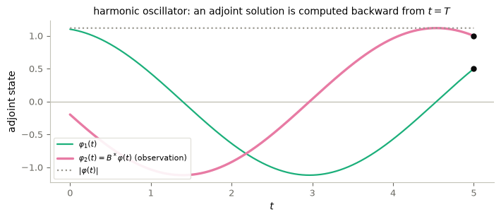
The black dots mark the terminal datum \(\varphi_T=(0.5,1)\), from which the solution is computed backward. Since \(A^*=-A\) is skew-symmetric, the adjoint rotates at the oscillator’s natural frequency, and \(|\varphi(t)|\) is constant. The observation \(B^*\varphi\) is therefore a sinusoid, \(B^*\varphi(t)=\varphi_{T,1}\sin(T-t)+\varphi_{T,2}\cos(T-t)\). Every control produced in this notebook will be such a curve.
3. The fundamental duality identity
We now derive the same identity without the explicit formula \(e^{At}\), using only the two differential equations. This second derivation matters because it carries over to time-dependent coefficients and to PDEs, where there is no matrix exponential but integration by parts still works.
Step 1. Differentiate the pairing. Let \(x\) solve the state equation with control \(u\), and let \(\varphi\) solve (ADJ). By the product rule, \[ \frac{d}{dt}\langle x(t),\varphi(t)\rangle=\langle x',\varphi\rangle+\langle x,\varphi'\rangle . \]
Step 2. Insert the equations. Using \(x'=Ax+Bu\) and \(\varphi'=-A^*\varphi\), \[ \frac{d}{dt}\langle x,\varphi\rangle=\langle Ax,\varphi\rangle+\langle Bu,\varphi\rangle-\langle x,A^*\varphi\rangle=\langle Bu,\varphi\rangle=\langle u,B^*\varphi\rangle . \] The terms with \(A\) cancel exactly: the adjoint is built so that they do. Only the control term survives.
Step 3. Integrate over \((0,T)\). For every \(\varphi_T\in\mathbb R^n\),
\[ \boxed{\;\langle x(T),\varphi_T\rangle-\langle x^0,\varphi(0)\rangle=\int_0^T\langle u(t),B^*\varphi(t)\rangle\,dt .\;} \tag{D} \]
Identity (D) is a conservation law with a source. Without control, the pairing \(\langle x(t),\varphi(t)\rangle\) is constant in time. The control changes it at the rate \(\langle u,B^*\varphi\rangle\).
Lemma 1 (controllability as a family of identities). Assumption: \(u\in L^2(0,T;\mathbb R^m)\).
Conclusion: \(u\) steers \(x^0\) to \(x^1\) if and only if, for every \(\varphi_T\in\mathbb R^n\), \[\int_0^T\langle u,B^*\varphi\rangle\,dt=\langle x^1,\varphi_T\rangle-\langle x^0,\varphi(0)\rangle .\tag{C}\]
Interpretation: a control is a solution of \(n\) linear equations, one for each basis direction \(\varphi_T=e_j\). The unknown \(u\) lives in an infinite-dimensional space.
Proof. By (D), condition (C) is equivalent to \(\langle x(T)-x^1,\varphi_T\rangle=0\) for every \(\varphi_T\). Taking \(\varphi_T=x(T)-x^1\) gives \(|x(T)-x^1|^2=0\). The converse is immediate. \(\square\)
Code and check. Verify (D) numerically for the harmonic oscillator, with an arbitrary control and an arbitrary test direction. Both sides are computed independently: the left side by simulating the state, the right side by quadrature along the adjoint.
x0 = torch.tensor([1.0, 0.0])                          # start: displaced, at rest
u_test = lambda s: torch.sin(3 * s).reshape(1)         # any control will do
phi_T_test = torch.tensor([1.0, 2.0])                  # any test direction will do

x_end = odeint(lti(A, B, u_test), x0, ts)[-1]
phi_test = adjoint(phi_T_test)
us_test = torch.stack([u_test(s) for s in ts])
lhs = x_end @ phi_T_test - x0 @ phi_test[0]
rhs = torch.trapezoid((us_test * (phi_test @ B)).sum(1), ts)
print(f"<x(T), phi_T> - <x0, phi(0)>  = {float(lhs):.6f}   (state simulation)")
print(f"int_0^T <u, B* phi> dt        = {float(rhs):.6f}   (quadrature along the adjoint)")
<x(T), phi_T> - <x0, phi(0)> = 0.341630 (state simulation)
int_0^T <u, B* phi> dt = 0.341628 (quadrature along the adjoint)4. From the identity to a functional
Condition (C) tells us which controls work, but not how to find one. The aim of this section is to turn (C) into a minimization problem. We do not pull a functional out of a hat: we reverse-engineer it from the equation we want its minimizer to satisfy.
Step 1. Look at (C) geometrically. In the Hilbert space \(L^2(0,T;\mathbb R^m)\) with inner product \((u,v)=\int_0^T\langle u,v\rangle\,dt\), the left side of (C) is \((u,B^*\varphi)\). Consider the set of functions \[ V=\{\,t\mapsto B^*\varphi(t)\;:\;\varphi_T\in\mathbb R^n\,\}\subset L^2(0,T;\mathbb R^m), \] a subspace of dimension at most \(n\). Condition (C) prescribes the inner products of \(u\) with the elements of \(V\), and with nothing else. Any component of \(u\) orthogonal to \(V\) is invisible to the constraints: it costs effort and achieves nothing. The most economical candidate is therefore a control lying in \(V\) itself:
\[ u=B^*\hat{\varphi}\quad\text{for some adjoint solution }\hat{\varphi}\text{ with terminal datum }\hat{\varphi}_T . \tag{ansatz} \]
(§7 proves that this candidate is the control of minimal norm.)
Step 2. Insert the ansatz into (C). We need \(\hat{\varphi}_T\) such that, for every \(\varphi_T\),
\[ \int_0^T\langle B^*\hat{\varphi},B^*\varphi\rangle\,dt=\langle x^1,\varphi_T\rangle-\langle x^0,\varphi(0)\rangle . \tag{EL} \]
The unknown is now a vector \(\hat{\varphi}_T\in\mathbb R^n\), not a function.
Step 3. Recognize (EL) as an optimality condition. The left side, \(a(\hat{\varphi}_T,\varphi_T):=\int_0^T\langle B^*\hat{\varphi},B^*\varphi\rangle\,dt\), is a symmetric bilinear form. The right side, \(\ell(\varphi_T):=\langle x^1,\varphi_T\rangle-\langle x^0,\varphi(0)\rangle\), is linear. For any symmetric bilinear \(a\) and linear \(\ell\), the directional derivative of \(\tfrac12a(\phi,\phi)-\ell(\phi)\) at \(\hat{\varphi}_T\) in a direction \(\varphi_T\) is \(a(\hat{\varphi}_T,\varphi_T)-\ell(\varphi_T)\). So (EL) says exactly that all directional derivatives of the following functional vanish at \(\hat{\varphi}_T\):
\[ \boxed{\;J(\varphi_T)=\frac12\int_0^T|B^*\varphi(t)|^2\,dt-\langle x^1,\varphi_T\rangle+\langle x^0,\varphi(0)\rangle,\qquad\varphi\text{ the solution of (ADJ)}.\;} \tag{HUM} \]
(EL) is the Euler–Lagrange equation of \(J\). We did not start from \(J\): we constructed it so that its critical points produce controls. In the literature this is the Hilbert Uniqueness Method (HUM) of J.-L. Lions.
Lemma 2 (minimizers give controls). Assumption: \(J\) has a minimizer \(\hat{\varphi}_T\).
Conclusion: \(u=B^*\hat{\varphi}\), where \(\hat{\varphi}\) solves (ADJ) with datum \(\hat{\varphi}_T\), steers \(x^0\) to \(x^1\).
Proof. At a minimizer of a differentiable function, all directional derivatives vanish, so (EL) holds. (EL) is (C) for \(u=B^*\hat{\varphi}\), and Lemma 1 concludes. \(\square\)
The whole difficulty has moved to one question: does \(J\) have a minimizer, and is it unique? The next section answers it, and the answer is observability.
5. Observability and coercivity
A function \(J:\mathbb R^n\to\mathbb R\) is coercive if \(J(z)\to+\infty\) as \(|z|\to\infty\), that is, if for every \(R\) there is \(\rho\) such that \(J(z)\ge R\) whenever \(|z|\ge\rho\). (Growth along each fixed ray is not enough.) The linear terms of \(J\) grow at most like \(|\varphi_T|\), so coercivity must come from the quadratic term \(\int_0^T|B^*\varphi|^2\). The argument has four links:
\[ \begin{aligned} &\text{unique continuation}\;\Longrightarrow\;\text{observability}\;\Longrightarrow\;\text{coercivity of }J,\\ &\text{continuity}+\text{coercivity}\;\Longrightarrow\;\text{existence of a minimizer},\\ &\text{strict convexity}\;\Longrightarrow\;\text{uniqueness}. \end{aligned} \]
(a) Unique continuation. If the observation \(B^*\varphi\) vanishes on all of \((0,T)\), then \(\varphi_T=0\). In words: the observation determines the adjoint state.
In finite dimension this is exactly Kalman’s condition. Differentiating \(B^*e^{A^*(T-t)}\varphi_T\equiv0\) repeatedly at \(t=T\) gives \(B^*(A^*)^k\varphi_T=0\) for all \(k\), that is, \(\varphi_T\perp\operatorname{Range}[B,AB,\dots,A^{n-1}B]\). Conversely, such \(\varphi_T\) make \(B^*\varphi\equiv0\), by the power series of the exponential and Cayley–Hamilton. Hence unique continuation ⟺ \(\operatorname{rank}\mathcal{K}(A,B)=n\).
(b) Observability. The adjoint system is observable in time \(T\) if there is \(c_0>0\) such that
\[ \int_0^T|B^*\varphi(t)|^2\,dt\;\ge\;c_0\,|\varphi(0)|^2\qquad\text{for every solution of (ADJ)}. \tag{OBS} \]
This is the quantitative version of unique continuation: a small observation forces a small state. We write \(c_0(T)\), or just \(c_0\), for the best constant; the subscript recalls that the state is measured at \(t=0\).
Measuring the state at the terminal time instead gives the terminal form \(\int_0^T|B^*\varphi|^2\ge c_{\rm term}|\varphi_T|^2\). In finite dimension the two forms are equivalent, because \(\varphi_T\mapsto\varphi(0)\) has a bounded inverse. With \(M=\|e^{-A^*T}\|\) we have \(|\varphi_T|\le M|\varphi(0)|\), hence \(c_{\rm term}\ge c_0/M^2\), and similarly \(c_0\ge c_{\rm term}/\|e^{A^*T}\|^2\).
Proposition 3. In finite dimension, unique continuation ⟺ observability.
Proof. “⇐”: if \(B^*\varphi\equiv0\), then (OBS) gives \(\varphi(0)=0\), hence \(\varphi_T=e^{-A^*T}\varphi(0)=0\).
“⇒”: the function \(Q(\varphi_T)=\int_0^T|B^*\varphi|^2\) is continuous and homogeneous of degree two. Restrict it to \(S=\{\varphi_T:|\varphi(0)|=1\}\), the preimage of the unit sphere under the invertible linear map \(\varphi_T\mapsto\varphi(0)\). \(S\) is compact, because it is closed and bounded in \(\mathbb R^n\) (Heine–Borel). By unique continuation \(Q>0\) on \(S\), and a continuous positive function on a compact set attains a positive minimum \(c_0\). For general \(\varphi_T\ne0\), apply this to \(\varphi_T/|\varphi(0)|\) and use homogeneity. \(\square\)
Where finite dimension is used. In two places: the compactness of \(S\) (unique continuation ⇒ observability), and the bounded inverse of \(\varphi_T\mapsto\varphi(0)\), which lets us pass between \(|\varphi(0)|\) and \(|\varphi_T|\). For the heat equation both fail (§11).
(c) Coercivity. From (OBS) and the Cauchy–Schwarz inequality, with \(|\varphi_T|\le M|\varphi(0)|\),
\[ \begin{aligned} J(\varphi_T)&\;\ge\;\frac{c_0}{2}|\varphi(0)|^2-\big(|x^0|+M|x^1|\big)\,|\varphi(0)|,\\ |\varphi(0)|&\;\ge\;\frac{|\varphi_T|}{\|e^{-A^*T}\|}=\frac{|\varphi_T|}{M}. \end{aligned} \]
The lower bound is \(g(|\varphi(0)|)\) with \(g(s)=\tfrac{c_0}{2}s^2-Ks\), \(K=|x^0|+M|x^1|\), and \(g\) is increasing for \(s\ge K/c_0\). Since \(|\varphi(0)|\ge|\varphi_T|/M\), we get \(J(\varphi_T)\ge g(|\varphi_T|/M)\) as soon as \(|\varphi_T|\ge MK/c_0\). Hence \(J(\varphi_T)\to+\infty\) as \(|\varphi_T|\to\infty\): \(J\) is coercive.
(d) Existence and uniqueness of the minimizer. Existence uses continuity and coercivity. Choose \(\rho\) such that \(J>J(0)=0\) outside the ball \(\{|\varphi_T|\le\rho\}\). On that ball, which is compact, the continuous function \(J\) attains its minimum, and this minimum is global. Uniqueness uses strict convexity: by (OBS), the quadratic part \(\tfrac12\int|B^*\varphi|^2\) is a positive definite quadratic form, so \(J\) is strictly convex, and a strictly convex function has at most one minimizer.
In infinite dimension, the compact-ball step is replaced by the direct method of the calculus of variations, which uses weak compactness.
6. Constructing the control
Putting §§3–5 together gives the main result of this notebook.
Theorem 4 (construction of controls by duality). Assumptions: \((A,B)\) satisfies the Kalman rank condition, equivalently unique continuation or observability of (ADJ). Let \(T>0\) and \(x^0,x^1\in\mathbb R^n\).
Conclusion: \(J\) has a unique minimizer \(\hat{\varphi}_T\), and \[\boxed{\;u(t)=B^*\hat{\varphi}(t)=B^*e^{A^*(T-t)}\hat{\varphi}_T\;}\] steers \(x^0\) to \(x^1\) in time \(T\).
Interpretation: the control is the observation of the optimal adjoint state. It belongs to the space \(V\), spanned by the \(n\) functions \(t\mapsto B^*e^{A^*(T-t)}e_j\), so it is determined by \(n\) numbers.
In one line: unique continuation → observability inequality → controllability, with a constructive procedure to build controls by minimizing a coercive functional.
The direction of the argument matters. Controllability, a property of the state equation, has been reduced to observability, a property of the adjoint equation. This is the precise meaning of the slogan “PRIMAL = DUAL, CONTROL = COMMUNICATION”: to control the system is to observe its adjoint.
For the harmonic oscillator, the figure of §2 already showed what such controls look like: sinusoids at the oscillator’s own frequency. The cheapest way to stop a swing is to push in resonance with it.
7. Why is this the minimum-\(L^2\) control?
Terminology. We call \(\|u\|_{L^2}=\big(\int_0^T|u|^2\big)^{1/2}\) the \(L^2\) effort of a control, and \(\tfrac12\|u\|_{L^2}^2\) its quadratic cost.
There are infinitely many controls: add to \(u\) any function orthogonal to \(V\). The heuristic in §4 suggested that the control in \(V\) is the most economical one. Here is the proof.
Theorem 5 (minimal norm). Assumptions: as in Theorem 4; \(\hat{u}=B^*\hat{\varphi}\) is the HUM control, and \(u\) is any control steering \(x^0\) to \(x^1\).
Conclusion: \(\|u\|_{L^2}^2=\|\hat{u}\|_{L^2}^2+\|u-\hat{u}\|_{L^2}^2\). Hence \(\|\hat{u}\|_{L^2}\le\|u\|_{L^2}\), with equality only if \(u=\hat{u}\).
Interpretation: \(\hat{u}\) is the orthogonal projection of \(0\) onto the affine set of all controls.
Proof. Both \(u\) and \(\hat{u}\) satisfy (C), which has the same right-hand side for both. Subtracting, \(\int_0^T\langle u-\hat{u},B^*\varphi\rangle\,dt=0\) for every \(\varphi_T\). Choosing \(\varphi_T=\hat{\varphi}_T\) gives \((u-\hat{u},\hat{u})_{L^2}=0\): the difference of two controls is orthogonal to the HUM control. Pythagoras then gives \[ \|u\|^2=\|\hat{u}+(u-\hat{u})\|^2=\|\hat{u}\|^2+2(\hat{u},u-\hat{u})+\|u-\hat{u}\|^2=\|\hat{u}\|^2+\|u-\hat{u}\|^2 .\qquad\square \]
The minimal quadratic cost and the minimum of \(J\). Taking \(\varphi_T=\hat{\varphi}_T\) in (EL) gives \(\|\hat{u}\|^2=\langle x^1,\hat{\varphi}_T\rangle-\langle x^0,\hat{\varphi}(0)\rangle\), so \(J(\hat{\varphi}_T)=\tfrac12\|\hat{u}\|^2-\|\hat{u}\|^2\). Therefore
\[ \min_{u:\,x(T)=x^1}\ \frac12\|u\|_{L^2}^2\;=\;-\min_{\varphi_T\in\mathbb R^n}J(\varphi_T). \]
The value of the dual problem gives the cost of the primal one, with the sign reversed. The laboratory checks this identity.
8. The Gramian interpretation
Let us compute \(J\) in matrix form. With \(\varphi(t)=e^{A^*(T-t)}\varphi_T\),
\[ \int_0^T|B^*\varphi|^2dt=\varphi_T^*\,\mathcal{G}_T\,\varphi_T, \qquad \langle x^0,\varphi(0)\rangle=\langle x^0,e^{A^*T}\varphi_T\rangle=\langle e^{AT}x^0,\varphi_T\rangle . \]
Hence, with \(d:=x^1-e^{AT}x^0\) (the part of the target that the free dynamics does not reach on its own),
\[ \boxed{\;J(\varphi_T)=\tfrac12\,\varphi_T^*\,\mathcal{G}_T\,\varphi_T-\langle d,\varphi_T\rangle,\qquad \nabla J(\varphi_T)=\mathcal{G}_T\varphi_T-d,\qquad \nabla^2J=\mathcal{G}_T .\;} \]
The Hessian of the HUM functional is the controllability Gramian. Let \(\lambda_1\le\dots\le\lambda_n\) be its eigenvalues with orthonormal eigenvectors \(q_j\). Three consequences follow.
- Formula (G) explained. The minimizer solves \(\mathcal{G}_T\hat{\varphi}_T=d\), so \(u=B^*e^{A^*(T-t)}\mathcal{G}_T^{-1}(x^1-e^{AT}x^0)\). The explicit control (G) is the HUM control, and therefore the minimal-norm control.
- Observability constants are eigenvalues. \(c_{\rm term}=\lambda_{\min}(\mathcal{G}_T)\), and \(c_0=\lambda_{\min}\big(e^{-AT}\mathcal{G}_Te^{-A^*T}\big)\). For the harmonic oscillator, \(e^{AT}\) is a rotation, so the two coincide.
- Cost of control, direction by direction. \[ \|\hat{u}\|_{L^2}^2=d^*\mathcal{G}_T^{-1}d=\sum_{j=1}^n\frac{|\langle d,q_j\rangle|^2}{\lambda_j}, \qquad \max_{|d|=1}\|\hat{u}\|_{L^2}=\lambda_{\min}(\mathcal{G}_T)^{-1/2}. \] A small \(\lambda_{\min}\) makes control expensive in the hard directions: those with a large component along the eigenvectors of small eigenvalues, and in the worst case. It does not make every target expensive; a target along an easy direction can remain cheap.
The speed of iterative minimization is a different matter: it is governed by the condition number \(\kappa(\mathcal{G}_T)=\lambda_{\max}/\lambda_{\min}\) (§10).
8.1 Reconstruction from noisy observations
Optional.
The Gramian also measures how stably the adjoint can be reconstructed from its observation. Define the observation operator
\[ \mathcal{O}_T:\mathbb R^n\to L^2(0,T;\mathbb R^m),\qquad (\mathcal{O}_Tz)(t)=B^*e^{A^*(T-t)}z, \qquad\text{so that}\qquad \mathcal{G}_T=\mathcal{O}_T^*\mathcal{O}_T . \]
Given the observation \(y=\mathcal{O}_T\varphi_T\), the least-squares reconstruction is \(\varphi_T=\mathcal{G}_T^{-1}\mathcal{O}_T^*y\). If the observation is corrupted, \(y+\delta y\), the reconstruction error is
\[ \delta\varphi_T=\mathcal{G}_T^{-1}\mathcal{O}_T^*\,\delta y, \qquad |\delta\varphi_T|\;\le\;\lambda_{\min}(\mathcal{G}_T)^{-1/2}\,\|\delta y\|_{L^2(0,T)} . \]
The constant is optimal, because the singular values of \(\mathcal{G}_T^{-1}\mathcal{O}_T^*\) are \(\lambda_j^{-1/2}\). The factor \(1/\lambda_{\min}\) would instead describe a perturbation \(\delta b\) of the right-hand side in the linear system \(\mathcal{G}_T\varphi_T=b\), which is a different question. For the harmonic oscillator with \(T=5\): \(\lambda_{\min}\approx2.0205\), so the noise gain is \(\lambda_{\min}^{-1/2}\approx0.7035\), not \(1/\lambda_{\min}\approx0.4949\).
Hard to observe and expensive to control are thus two readings of the same eigenvalues, seen from the two sides of the duality.
9. Computational laboratory
We test the chain on two examples: the harmonic oscillator (everything computed, and HUM compared with formula (G)) and a near-uncontrollable family (observability, conditioning and cost degrade together).
9.1 The harmonic oscillator, step by step
We stop the oscillator: start displaced and at rest, \(x^0=(1,0)\), and arrive at rest at the origin, \(x^1=(0,0)\), at time \(T=5\), which is less than one period \(2\pi\).
Code and check. The Kalman matrix, the Gramian and the observability constants of the oscillator.
x1 = torch.tensor([0.0, 0.0])                          # target: at rest at the origin

K = kalman(A, B)
print("Kalman matrix K = [B, AB] =\n", K.numpy())
print("rank K =", int(torch.linalg.matrix_rank(K)), "= n, so (A, B) is controllable "
      "(unique continuation holds)")

G = gramian(A, B, T)
lam = torch.linalg.eigvalsh(G)
lam_exact = torch.tensor([T - abs(np.sin(T)), T + abs(np.sin(T))]) / 2     # closed form, Exercise 3
c_term = float(lam[0])
c_0 = float(torch.linalg.eigvalsh(torch.matrix_exp(-A * T) @ G @ torch.matrix_exp(-A.T * T))[0])
print("\nGramian G_T =\n", G.numpy().round(6))
print("eigenvalues (quadrature):  ", lam.numpy())
print("eigenvalues (closed form): ", lam_exact.numpy())
print(f"c_0 = {c_0:.8f}   c_term = {c_term:.8f}   (equal: e^(AT) is a rotation)")
Kalman matrix K = [B, AB] =
[[0. 1.]
[1. 0.]]
rank K = 2 = n, so (A, B) is controllable (unique continuation holds)
Gramian G_T =
[[2.635998 0.459744]
[0.459744 2.364002]]
eigenvalues (quadrature): [2.02056283 2.97943717]
eigenvalues (closed form): [2.02053786 2.97946214]
c_0 = 2.02056283 c_term = 2.02056283 (equal: e^(AT) is a rotation)Optional check: the constant as a minimum over a compact set. Proposition 3 obtained \(c_0\) as the minimum of the observation energy over \(S=\{|\varphi(0)|=1\}\). Random points of \(S\) give ratios \(\int|B^*\varphi|^2/|\varphi(0)|^2\) that approach \(c_0\) from above and never go below it.
phi0_samples = torch.randn(20000, 2)
phi0_samples /= phi0_samples.norm(dim=1, keepdim=True)
phiT_samples = phi0_samples @ torch.matrix_exp(-A * T)         # rows: phi_T = e^{-A^T T} phi(0)
energies = torch.einsum("ij,jk,ik->i", phiT_samples, G, phiT_samples)
print(f"smallest sampled ratio over 20000 random points of S = {float(energies.min()):.8f}")
print(f"c_0                                                  = {c_0:.8f}")
smallest sampled ratio over 20000 random points of S = 2.02056284
c_0 = 2.02056283The HUM minimizer, computed two independent ways.
- Route 1, the dual problem as stated. Minimize \(J(\varphi_T)\) numerically, evaluating \(J\) only through adjoint trajectories — no Gramian is used. The gradient comes from automatic differentiation through the quadrature, and L-BFGS does the minimization. We check that the gradient vanishes at the result.
- Route 2, the Gramian identity of §8. Solve \(\mathcal{G}_T\hat{\varphi}_T=x^1-e^{AT}x^0\).
From the Route 1 minimizer we then build \(\hat{u}=B^*\hat{\varphi}\), simulate the controlled system, and compare \(\hat{u}\) with formula (G).
def J_dual(phi_T):
    """J evaluated through the adjoint trajectory only (no Gramian)."""
    phi = Es @ phi_T                                   # the whole adjoint trajectory
    obs = (phi @ B).squeeze(-1)                        # B* phi(t)
    return 0.5 * torch.trapezoid(obs ** 2, ts) - x1 @ phi_T + x0 @ phi[0]

# Route 1: L-BFGS on J, gradients by automatic differentiation.
phi_hat = torch.zeros(2, requires_grad=True)
opt = torch.optim.LBFGS([phi_hat], max_iter=100, tolerance_grad=1e-14,
                        tolerance_change=1e-16, line_search_fn="strong_wolfe")
opt.step(lambda: (opt.zero_grad(), loss := J_dual(phi_hat), loss.backward(), loss)[1])
residual = torch.autograd.grad(J_dual(phi_hat), phi_hat)[0].norm()
phi_T_hum = phi_hat.detach()

# Route 2: the linear system G_T phi_T = x1 - e^{AT} x0.
phi_T_gram = torch.linalg.solve(G, x1 - torch.matrix_exp(A * T) @ x0)

# The control from Route 1, formula (G), and the controlled trajectory.
hum_control = lambda phi_T: lambda t: B.T @ torch.matrix_exp(A.T * (T - t)) @ phi_T
u_hum = ((Es @ phi_T_hum) @ B).squeeze(-1)             # sampled on the grid
u_G = ((Es @ phi_T_gram) @ B).squeeze(-1)
x_traj = odeint(lti(A, B, hum_control(phi_T_hum)), x0, ts)
phi_traj = Es @ phi_T_hum
cost = 0.5 * float(torch.trapezoid(u_hum ** 2, ts))

print("minimizer, route 1 (L-BFGS on J):", phi_T_hum.numpy(), "  route 2 (Gramian):", phi_T_gram.numpy())
print("\nDiagnostics")
print(f"  optimality residual |grad J(phi_hat)|        = {float(residual):.1e}")
print(f"  |phi_hat(route 1) - phi_hat(route 2)|        = {float((phi_T_hum - phi_T_gram).norm()):.1e}")
print(f"  max_t |u_HUM(t) - u_G(t)|                    = {float((u_hum - u_G).abs().max()):.1e}")
print(f"  terminal error |x(T) - x1|                   = {float((x_traj[-1] - x1).norm()):.1e}")
print(f"  quadratic cost 1/2 ||u_HUM||^2               = {cost:.10f}")
print(f"  -min J                                       = {-float(J_dual(phi_T_hum)):.10f}")
minimizer, route 1 (L-BFGS on J): [-0.03815446 -0.39821663] route 2 (Gramian): [-0.0381583 -0.39821511]
Diagnostics
optimality residual |grad J(phi_hat)| = 4.1e-16
|phi_hat(route 1) - phi_hat(route 2)| = 4.1e-06
max_t |u_HUM(t) - u_G(t)| = 4.1e-06
terminal error |x(T) - x1| = 4.0e-07
quadratic cost 1/2 ||u_HUM||^2 = 0.1963412837
-min J = 0.1963412837Both routes give the same minimizer, and the HUM control agrees with formula (G) to the accuracy of the quadrature. The controlled state reaches the target, and \(-\min J\) reproduces the quadratic cost (§7).
The free oscillator conserves its energy \(E=\tfrac12|x|^2\). Under the HUM control the energy must go from \(\tfrac12\) to \(0\) — but does it decrease monotonically?
Code and plot. The controlled trajectory in the phase plane, and the state and energy against time.
s = np.linspace(0, 2 * np.pi, 300)
fig, (ax1, ax2) = P.panels(2, size=(4.4, 3.5))

ax1.plot(np.cos(s), -np.sin(s), ":", color=P.GREY, label="free motion $e^{At}x^0$")
ax1.plot(x_traj[:, 0], x_traj[:, 1], color=P.BLUE, label="controlled trajectory")
ax1.plot(*x0, "o", color=P.INK); ax1.annotate("$x^0$", x0, xytext=(5, 5), textcoords="offset points")
ax1.plot(*x1, "*", ms=12, color=P.ORANGE); ax1.annotate("$x^1$", x1, xytext=(5, -12), textcoords="offset points")
P.label(ax1, "position $x_1$", "velocity $x_2$", title="phase plane", equal=True, xlim=(-1.15, 1.9))

P.curves(ax2, ts, {"$x_1(t)$ (position)": (x_traj[:, 0], P.BLUE),
                   "$x_2(t)$ (velocity)": (x_traj[:, 1], P.AQUA),
                   r"energy $\frac{1}{2}|x(t)|^2$": (0.5 * (x_traj ** 2).sum(1),
                                                     {"color": P.GREY, "ls": "--"})},
         xlabel="$t$", ylabel="state", zero="h", title="state components")
plt.show()

energy_rising = float(torch.mean((x_traj[:, 1] * u_hum > 0).double()))     # E'(t) = x2(t) u(t)
print(f"fraction of the horizon in which the energy increases: {energy_rising:.1%}")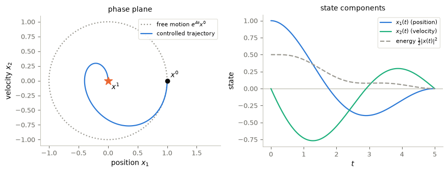
fraction of the horizon in which the energy increases: 12.3%The control does not fight the dynamics. It lets the oscillator swing and removes its energy, bringing the state to rest exactly at \(t=T\). Since \(E'(t)=x_2(t)\,u(t)\), energy is removed when the control opposes the velocity. This happens most of the time, but not always: during about 12% of the horizon the energy increases slightly. The minimal-\(L^2\) control optimizes the total effort under an exact terminal constraint, not the energy loss at each instant. An autonomous linear feedback produces asymptotic decay and cannot reach the equilibrium in finite time from a nonzero initial state.
Code and plot. The HUM control against formula (G), and the optimal adjoint behind both.
fig, (ax1, ax2) = P.panels(2, size=(4.4, 3.3))
P.curves(ax1, ts, {r"HUM: $\hat{u}=B^*\hat{\varphi}$": (u_hum, P.ORANGE),
                   "formula (G)": (u_G, {"color": P.INK, "ls": "--", "lw": 1.0})},
         xlabel="$t$", ylabel="$u(t)$", zero="h", title="the control")
P.curves(ax2, ts, {r"$\hat{\varphi}_1(t)$": (phi_traj[:, 0], P.AQUA),
                   r"$\hat{\varphi}_2(t)=B^*\hat{\varphi}(t)$": (phi_traj[:, 1],
                                                                 {"color": P.MAGENTA, "lw": 2.4})},
         xlabel="$t$", ylabel="adjoint state", zero="h",
         title=r"the optimal adjoint $\hat{\varphi}$")
ax2.plot([T, T], phi_T_hum, "o", color=P.INK, ms=5)
plt.show()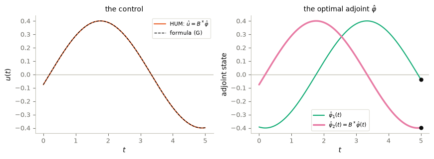
The two controls coincide (difference at rounding level, see the diagnostics): formula (G) is the minimal-norm HUM control (§8). The control is the observed component \(\hat{\varphi}_2\) of the optimal adjoint, the same curve in both panels, and it is determined by two numbers, \(\hat{\varphi}_T\in\mathbb R^2\).
9.2 The near-uncontrollable family: losing controllability
Now consider the family \[ A=\begin{pmatrix}0&1&0\\-1&0&0\\0&0&-1\end{pmatrix},\qquad B_\varepsilon=\begin{pmatrix}0\\1\\\varepsilon\end{pmatrix}. \] It couples the oscillator to a decaying mode \(x_3'=-x_3+\varepsilon u\), which the actuator reaches only with strength \(\varepsilon\). Its Kalman determinant is \(-2\varepsilon\), so the pair is controllable if and only if \(\varepsilon\ne0\).
We take \(x^0=0\) and \(x^1=e_3\), so \(d=e_3\): we must excite the weakly actuated mode. As \(\varepsilon\to0\), how do \(\lambda_{\min}(\mathcal{G}_T)\), the condition number \(\kappa(\mathcal{G}_T)\) and the minimal \(L^2\) effort \(\|\hat{u}\|_{L^2}\) behave?
Code and plot. Sweep \(\varepsilon\), and compute the constant \(\sigma_T\) of the predicted rates (derived in §9.2a below): the squared \(L^2(0,T)\)-distance from \(r\mapsto e^{-r}\) to \(\operatorname{span}\{\sin r,\cos r\}\).
def family(eps):
    A2 = torch.tensor([[0.0, 1.0, 0.0], [-1.0, 0.0, 0.0], [0.0, 0.0, -1.0]])
    return A2, torch.tensor([[0.0], [1.0], [eps]])

epsilons = np.logspace(-3, 0, 13)
d = torch.tensor([0.0, 0.0, 1.0])                      # x0 = 0, x1 = e3
lam_min, cond, u_norm = [], [], []
for eps in epsilons:
    G2 = gramian(*family(float(eps)), T)
    ev = torch.linalg.eigvalsh(G2)
    lam_min.append(float(ev[0]))
    cond.append(float(ev[-1] / ev[0]))
    u_norm.append(float(torch.sqrt(d @ torch.linalg.solve(G2, d))))    # ||u_hat|| (Section 8)
lam_min, cond, u_norm = map(np.array, (lam_min, cond, u_norm))

# sigma_T: squared L^2-distance from e^{-r} to span{sin r, cos r}; note G_osc = the oscillator Gramian G
r = torch.linspace(0, T, 4001)
w = torch.stack([torch.sin(r), torch.cos(r)])          # w(r) = e^{A_osc r} b_osc
g = torch.trapezoid(torch.exp(-r) * w, r, dim=1)
gamma = torch.trapezoid(torch.exp(-2 * r), r)
sigma_T = float(gamma - g @ torch.linalg.solve(G, g))
print(f"sigma_T = {sigma_T:.6f}")

fig, axes = P.panels(3, size=(3.8, 3.3))
axes[0].loglog(epsilons, lam_min, "o-", color=P.BLUE, label=r"$\lambda_{\min}(\mathcal{G}_T)=c_{\rm term}$")
axes[0].loglog(epsilons, sigma_T * epsilons ** 2, "--", color=P.NOTE, lw=1, label=r"$\sigma_T\,\varepsilon^2$")
P.label(axes[0], r"actuator strength $\varepsilon$", title="terminal observability constant")
axes[1].loglog(epsilons, cond, "o-", color=P.AQUA, label=r"$\kappa(\mathcal{G}_T)$")
axes[1].loglog(epsilons, cond[-1] * (epsilons / epsilons[-1]) ** -2.0, "--", color=P.NOTE, lw=1,
               label="slope $-2$")
P.label(axes[1], r"actuator strength $\varepsilon$", title="condition number")
axes[2].loglog(epsilons, u_norm, "o-", color=P.ORANGE, label=r"$\|\hat{u}\|_{L^2}$ for $d=e_3$")
axes[2].loglog(epsilons, 1 / (np.sqrt(sigma_T) * epsilons), "--", color=P.NOTE, lw=1,
               label=r"$1/(\varepsilon\sqrt{\sigma_T})$")
P.label(axes[2], r"actuator strength $\varepsilon$", title=r"$L^2$ effort of the minimal control")
plt.show()
sigma_T = 0.331308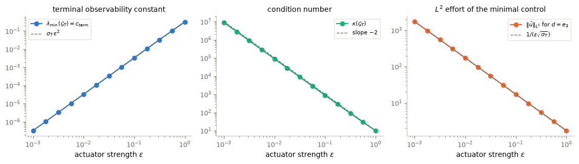
The system is controllable for every \(\varepsilon>0\); Kalman’s rank test says yes throughout. Yet the terminal observability constant behaves like \(\varepsilon^2\), the condition number like \(\varepsilon^{-2}\), and the effort needed to reach \(e_3\), a hard direction, like \(\varepsilon^{-1}\). Controllability is a yes/no property; observability constants measure how controllable a system is.
The dashed lines rest on two facts proved below: \(\|\hat{u}\|_{L^2}=1/(\varepsilon\sqrt{\sigma_T})\) exactly, and \(\lambda_{\min}(\mathcal{G}_T)/\varepsilon^2\to\sigma_T\) as \(\varepsilon\to0\).
9.2a Why these rates? (Schur complement)
Optional.
Here \(e^{Ar}B_\varepsilon=(w(r),\varepsilon e^{-r})\) with \(w(r)=(\sin r,\cos r)\), the oscillator’s response. Writing \(D_\varepsilon=\operatorname{diag}(1,1,\varepsilon)\), the Gramian factorizes as
\[ \mathcal{G}_T(\varepsilon)=D_\varepsilon\,H\,D_\varepsilon,\qquad H=\begin{pmatrix}G_{\rm osc}&g\\ g^*&\gamma\end{pmatrix},\quad G_{\rm osc}=\int_0^Tww^*,\quad g=\int_0^Te^{-r}w(r)\,dr,\quad\gamma=\int_0^Te^{-2r}dr, \]
where \(H=\mathcal{G}_T(1)\) is positive definite and does not depend on \(\varepsilon\).
Exact effort. By the block-inverse (Schur complement) formula, \((H^{-1})_{33}=1/\sigma_T\) with \(\sigma_T=\gamma-g^*G_{\rm osc}^{-1}g\). Since \(\mathcal{G}_T(\varepsilon)^{-1}=D_\varepsilon^{-1}H^{-1}D_\varepsilon^{-1}\), we get \(e_3^*\mathcal{G}_T(\varepsilon)^{-1}e_3=1/(\varepsilon^2\sigma_T)\), that is, \(\|\hat{u}\|_{L^2}=1/(\varepsilon\sqrt{\sigma_T})\) for every \(\varepsilon>0\).
Asymptotics of \(\lambda_{\min}\). The matrix \(\varepsilon^2\mathcal{G}_T(\varepsilon)^{-1}=\varepsilon^2D_\varepsilon^{-1}H^{-1}D_\varepsilon^{-1}\) has entries \(\varepsilon^2(H^{-1})_{ij}\) in the \(2\times2\) block, \(\varepsilon(H^{-1})_{i3}\) in the last row and column, and \((H^{-1})_{33}=1/\sigma_T\) in the corner. As \(\varepsilon\to0\) it converges to \(\operatorname{diag}(0,0,1/\sigma_T)\). Eigenvalues depend continuously on the matrix, so \(\varepsilon^2\lambda_{\max}(\mathcal{G}_T(\varepsilon)^{-1})\to1/\sigma_T\), that is, \[ \lambda_{\min}(\mathcal{G}_T(\varepsilon))/\varepsilon^2\;\longrightarrow\;\sigma_T\qquad(\varepsilon\to0,\ T\text{ fixed}). \] The other two eigenvalues of \(\mathcal{G}_T(\varepsilon)\) converge to those of \(G_{\rm osc}\), so \(\kappa\sim\lambda_{\max}(G_{\rm osc})/(\sigma_T\varepsilon^2)\).
The two observability constants. For this family, \(e^{AT}\) is not a rotation, so \(c_0\) and \(c_{\rm term}\) differ. The same argument applied to \(e^{-AT}\mathcal{G}_Te^{-A^*T}\), whose third row and column are scaled by \(\varepsilon e^{T}\) instead of \(\varepsilon\), gives \(c_0/\varepsilon^2\to\sigma_Te^{2T}\). Hence \(c_0/c_{\rm term}\to e^{2T}\) as \(\varepsilon\to0\) with \(T\) fixed. The weak mode decays by itself, so driving it to zero (null control, measured by \(c_0\)) is much cheaper than exciting it (our target \(e_3\), measured by \(c_{\rm term}\)). The table below confirms these limits numerically; it illustrates the proof but does not replace it.
print("eps      lambda_min/eps^2   eps*||u_hat||   c_0/(eps^2 e^{2T})   c_0/c_term")
for eps in [1.0, 0.1, 0.01, 0.001]:
    A2, B2 = family(eps)
    G2 = gramian(A2, B2, T)
    ct = float(torch.linalg.eigvalsh(G2)[0])
    c0 = float(torch.linalg.eigvalsh(torch.matrix_exp(-A2 * T) @ G2 @ torch.matrix_exp(-A2.T * T))[0])
    eff = float(torch.sqrt(d @ torch.linalg.solve(G2, d)))
    print(f"{eps:6.3f}   {ct / eps**2:14.6f}   {eps * eff:12.6f}   {c0 / (eps**2 * np.exp(2 * T)):16.6f}"
          f"   {c0 / ct:10.1f}")
print(f"limits:  sigma_T = {sigma_T:.6f},  1/sqrt(sigma_T) = {1 / np.sqrt(sigma_T):.6f},"
      f"  e^(2T) = {np.exp(2 * T):.1f}")
eps lambda_min/eps^2 eps*||u_hat|| c_0/(eps^2 e^{2T}) c_0/c_term
1.000 0.311348 1.737272 0.000085 6.0
0.100 0.331143 1.737272 0.008425 560.4
0.010 0.331331 1.737272 0.285381 18971.7
0.001 0.331333 1.737272 0.330914 21998.6
limits: sigma_T = 0.331308, 1/sqrt(sigma_T) = 1.737338, e^(2T) = 22026.510. Optimization preview: conditioning slows gradient descent
The dual functional is a quadratic with Hessian \(\mathcal{G}_T\). Suppose we minimize it by gradient descent (GD), \[ \varphi_T^{(k+1)}=\varphi_T^{(k)}-\eta\,\nabla J\big(\varphi_T^{(k)}\big),\qquad\nabla J(\varphi_T)=\mathcal{G}_T\varphi_T-d . \]
The gradient has a meaning. By the variation-of-constants formula, the state driven by \(u=B^*\varphi\) from \(x^0\) ends at \(x_\varphi(T)=e^{AT}x^0+\mathcal{G}_T\varphi_T\). Hence
\[ \nabla J(\varphi_T)=x_\varphi(T)-x^1 : \]
the gradient of the dual functional is the terminal miss. Each gradient step means: apply the control \(B^*\varphi\), see by how much the target is missed, and correct the adjoint datum. It costs one adjoint solve and one state solve, and needs no Gramian (Exercise 5).
Speed depends on the condition number, not on \(\lambda_{\min}\) alone. The error \(e_k=\varphi_T^{(k)}-\hat{\varphi}_T\) obeys \(e_{k+1}=(I-\eta\mathcal{G}_T)e_k\). With \(\eta=1/\lambda_{\max}\), the component along \(q_j\) is multiplied by \(1-\lambda_j/\lambda_{\max}\) per step. The slowest mode, along \(q_1\), contracts by \(1-1/\kappa\), with \(\kappa=\kappa(\mathcal{G}_T)\). For large \(\kappa\) this gives the worst-case estimate \[ k\;\approx\;\kappa\,\ln(1/\delta) \] for the number of steps needed to reduce the error by a factor \(\delta\). The actual count depends on how much of the initial error lies along the slow modes. A small \(\lambda_{\min}\) alone does not make GD slow: for \(\mathcal{G}=\varepsilon^2I\), controls are expensive for small \(\varepsilon\), yet \(\kappa=1\) and GD with \(\eta=1/\lambda_{\max}\) solves the problem in one step. For the near-uncontrollable family, \(\kappa\sim\varepsilon^{-2}\), and GD becomes slow.
Code and plot. Check that the gradient is the terminal miss, then run GD on the dual functional of the oscillator and of the near-uncontrollable family for several \(\varepsilon\).
# The gradient of J is the terminal miss (the oscillator, an arbitrary phi_T):
phi_check = torch.tensor([0.3, -0.7])
x_end = odeint(lti(A, B, hum_control(phi_check)), x0, ts)[-1]
print("G phi - d     =", (G @ phi_check - (x1 - torch.matrix_exp(A * T) @ x0)).numpy())
print("x_phi(T) - x1 =", (x_end - x1).numpy())

def gradient_descent_hum(G, d, tol=1e-6, max_iter=500_000):
    # phi_{k+1} = phi_k - eta (G phi_k - d), eta = 1/lambda_max, from phi_0 = 0.
    # Stops at the first k with |phi_k - phi_hat| <= tol |phi_hat|; returns the relative errors.
    phi_star = torch.linalg.solve(G, d)
    eta = 1.0 / torch.linalg.eigvalsh(G)[-1]
    phi = torch.zeros_like(d)
    errors = [1.0]
    while errors[-1] > tol:
        if len(errors) > max_iter:
            raise RuntimeError(f"gradient descent did not reach tol={tol} in {max_iter} steps")
        phi = phi - eta * (G @ phi - d)
        errors.append(float((phi - phi_star).norm() / phi_star.norm()))
    return np.array(errors)

print("\nG = eps^2 I (expensive controls, kappa = 1):",
      len(gradient_descent_hum(1e-4 * torch.eye(3), d)) - 1, "step")

cases = {"oscillator": (G, x1 - torch.matrix_exp(A * T) @ x0)}
for eps in [1.0, 0.3, 0.1, 0.03]:
    cases[f"family, eps={eps}"] = (gramian(*family(eps), T), d)

runs = {name: (float(torch.linalg.cond(Gc)), gradient_descent_hum(Gc, dc))
        for name, (Gc, dc) in cases.items()}
for name, (kappa, errs) in runs.items():
    print(f"{name:16s} kappa = {kappa:10.1f}   steps to 1e-6: {len(errs) - 1:7d}"
          f"   worst-case estimate kappa*ln(1e6) = {kappa * np.log(1e6):9.0f}")
G phi - d = [ 0.75264089 -0.55795381]
x_phi(T) - x1 = [ 0.75262625 -0.55794167]
G = eps^2 I (expensive controls, kappa = 1): 1 step
oscillator kappa = 1.5 steps to 1e-6: 12 worst-case estimate kappa*ln(1e6) = 20
family, eps=1.0 kappa = 10.2 steps to 1e-6: 134 worst-case estimate kappa*ln(1e6) = 140
family, eps=0.3 kappa = 100.9 steps to 1e-6: 1388 worst-case estimate kappa*ln(1e6) = 1395
family, eps=0.1 kappa = 900.2 steps to 1e-6: 12431 worst-case estimate kappa*ln(1e6) = 12437
family, eps=0.03 kappa = 9992.4 steps to 1e-6: 138044 worst-case estimate kappa*ln(1e6) = 138051fig, (ax1, ax2) = P.panels(2, size=(4.4, 3.4))
for name, (kappa, errs) in runs.items():
ax1.loglog(np.arange(1, len(errs) + 1), errs, label=rf"{name} ($\kappa\approx${kappa:.3g})")
P.label(ax1, "iteration $k$ (+1)", r"$|\varphi_T^{(k)}-\hat{\varphi}_T|/|\hat{\varphi}_T|$",
title="gradient descent on $J$")
kappas = np.array([v[0] for v in runs.values()])
iters = np.array([len(v[1]) - 1 for v in runs.values()])
ax2.loglog(kappas, iters, "o", color=P.BLUE, label="observed")
kk = np.logspace(0, np.log10(kappas.max()) + 0.2, 50)
ax2.loglog(kk, kk * np.log(1e6), "--", color=P.GREY, label=r"worst case $\kappa\,\ln(10^6)$")
P.label(ax2, r"condition number $\kappa(\mathcal{G}_T)$", "steps to $10^{-6}$",
title="cost of computing the control")
plt.show()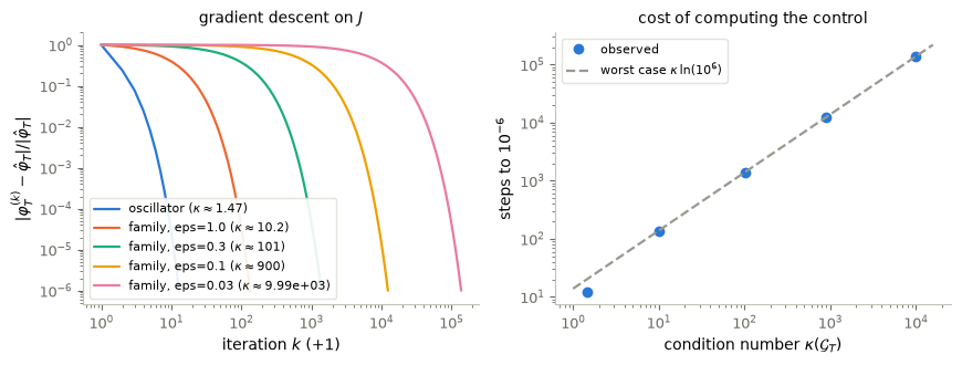
For the oscillator (\(\kappa\approx1.5\)) about a dozen steps suffice, fewer than the worst-case estimate. For the near-uncontrollable family the target \(e_3\) lies almost along the slow mode, so the estimate is nearly attained, and each tenfold decrease of \(\varepsilon\) multiplies \(\kappa\), and the number of steps, by about one hundred: conditioning of the dual problem → speed of iterative solvers.
11. What changes in infinite dimension?
Optional.
Finite dimension entered the chain in two places (§5): compactness of the unit sphere, and the bounded inverse of \(\varphi_T\mapsto\varphi(0)\). Here is what goes wrong without them.
Injective does not imply bounded below. On \(\ell^2\), the diagonal operator \((Lv)_k=v_k/k\) is injective, the analogue of unique continuation, but not bounded below: \(|e_k|=1\) while \(|Le_k|=1/k\to0\). The proof of Proposition 3 breaks exactly where expected. The sequence \((e_k)\) lies on the unit sphere but has no convergent subsequence (\(|e_j-e_k|=\sqrt2\)), so the infimum \(0\) of \(|Lv|\) over the sphere is not attained.
The heat equation: three different operators. In this section \(x\in(0,1)\) denotes the spatial variable. Consider the adjoint heat equation \(-\varphi_t-\varphi_{xx}=0\) on \((0,1)\) with Dirichlet conditions and \(\varphi(T)=\varphi_T\), observed on the whole interval, \(\omega=(0,1)\). In the eigenbasis \(e_k\) of \(-\partial_{xx}\), with eigenvalues \(\lambda_k=k^2\pi^2\), each mode evolves independently, and three operators must be kept apart.
- The semigroup \(S_T:\varphi_T\mapsto\varphi(0)\), with \(S_Te_k=e^{-\lambda_kT}e_k\). It is injective, but \(s_{\min}\) of its \(N\)-mode truncation is \(e^{-\lambda_NT}\). This is not an observability constant.
- The observation operator \(\mathcal{O}_T:\varphi_T\mapsto\varphi|_{(0,T)\times\omega}\). Here \[ \|\mathcal{O}_Te_k\|^2_{L^2((0,T)\times(0,1))}=\int_0^Te^{-2\lambda_k(T-t)}dt=\frac{1-e^{-2\lambda_kT}}{2\lambda_k}. \]
- The Gramian \(\mathcal{G}_T=\mathcal{O}_T^*\mathcal{O}_T\), which is diagonal with exactly these entries.
For the \(N\)-mode truncation, the entries above decrease with \(\lambda\), so \[ s_{\min}(\mathcal{O}_{T,N})=\sqrt{\frac{1-e^{-2\lambda_NT}}{2\lambda_N}}\sim\frac1{\sqrt2\,\pi N}, \qquad c_{\rm term}(N)=\lambda_{\min}(\mathcal{G}_{T,N})=\frac{1-e^{-2\lambda_NT}}{2\lambda_N}\sim\frac1{2\pi^2N^2}. \] These decay polynomially, like \(N^{-1}\) and \(N^{-2}\). The exponential decay of \(S_T\) does not transfer to the Gramian, and one should not infer exponential rates for heat-control Gramians from it.
In any case \(c_{\rm term}(N)\to0\), so the terminal form of observability is impossible for the heat equation, even with observation on the whole domain.
The initial form (OBS) behaves differently. Mode by mode, the ratio \(\|\mathcal{O}_Te_k\|^2/|S_Te_k|^2=(e^{2\lambda_kT}-1)/(2\lambda_k)\) increases with \(k\), so \[ \int_0^T\!\!\int_0^1|\varphi|^2\,dx\,dt\;\ge\;c_0\,|\varphi(0)|^2,\qquad c_0=\frac{e^{2\pi^2T}-1}{2\pi^2}>0, \] uniformly in \(N\). The two forms of observability, equivalent in finite dimension, now give different answers, because \(S_T\) has no bounded inverse.
That form corresponds to null controllability. For observation on the whole domain it is elementary, as above. For a proper subset \(\omega\subsetneq(0,1)\) it is a deep theorem (Fursikov–Imanuvilov, Lebeau–Robbiano), whose proof requires additional quantitative estimates, for example Carleman estimates or spectral methods. Compactness can no longer do the job.
Code and plot. The closed-form constants of the truncated heat problem, against the number of modes.
N = np.arange(1, 201)
T_heat = 0.05
lam_k = (np.pi * N) ** 2
g_term = -np.expm1(-2 * lam_k * T_heat) / (2 * lam_k)        # lambda_min(G_{T,N}) = c_term(N)
s_obs = np.sqrt(g_term)                                       # s_min(O_{T,N})
c0_heat = np.expm1(2 * np.pi ** 2 * T_heat) / (2 * np.pi ** 2)    # c_0, attained by the first mode

fig, ax = P.panels(figsize=(6.8, 3.6))
ax.loglog(N, 1.0 / N, color=P.BLUE, label=r"$\ell^2$ example: $s_{\min}=1/N$")
ax.loglog(N, s_obs, color=P.ORANGE, label=r"heat: $s_{\min}(\mathcal{O}_{T,N})$")
ax.loglog(N, g_term, "--", color=P.ORANGE, label=r"heat: $c_{\rm term}(N)=\lambda_{\min}(\mathcal{G}_{T,N})$")
ax.loglog(N, np.full_like(N, c0_heat, dtype=float), ":", color=P.INK, label=r"heat: $c_0$ (initial form)")
P.label(ax, "number $N$ of modes in the truncation", "constant",
        title=r"heat equation, $\omega=(0,1)$, $T=0.05$: two forms of observability")
plt.show()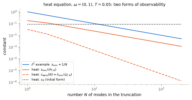
Every truncation is injective, and the terminal constant is positive for each \(N\). But it tends to zero, like \(N^{-2}\), so no single constant works in infinite dimension. The initial constant \(c_0\) stays bounded away from zero. In finite dimension the two forms of observability were equivalent; for the heat equation one holds and the other fails. (The semigroup \(S_T\) is not plotted: its singular values \(e^{-\lambda_kT}\) are not observability constants.)
12. Control ↔︎ ML connection
The adjoint propagates sensitivity information backwards. In §1, \(B^*\varphi(s)\) was the derivative of \(\langle x(T),\varphi_T\rangle\) with respect to the control at time \(s\), obtained by one backward solve. The same structural idea will reappear as backpropagation: a residual network is a discretized controlled ODE whose parameters play the role of \(u\), and the gradient of the loss with respect to all parameters comes from one backward adjoint sweep. Backpropagation is reverse-mode differentiation.
Key takeaways
- Testing \(x(T)\) against every direction \(\varphi_T\) turns reachability into scalar identities, and the adjoint system \(-\varphi'=A^*\varphi\), \(\varphi(T)=\varphi_T\), appears by itself.
- Duality identity: \(\langle x(T),\varphi_T\rangle-\langle x^0,\varphi(0)\rangle=\int_0^T\langle u,B^*\varphi\rangle\,dt\).
- The HUM functional \(J(\varphi_T)=\tfrac12\int_0^T|B^*\varphi|^2-\langle x^1,\varphi_T\rangle+\langle x^0,\varphi(0)\rangle\) is reverse-engineered so that its Euler–Lagrange equation is the control condition.
- Unique continuation ⇒ observability ⇒ coercivity ⇒ existence; strict convexity ⇒ uniqueness. Finite dimension enters through compactness and a bounded inverse.
- The control is the observation of the optimal adjoint, \(\hat{u}=B^*\hat{\varphi}\). It has minimal \(L^2\) effort, and \(\min\tfrac12\|u\|^2=-\min J\).
- \(\nabla^2J=\mathcal{G}_T\): the explicit Gramian control is the HUM control.
- \(\|\hat{u}\|^2=\sum_j|\langle d,q_j\rangle|^2/\lambda_j\): small eigenvalues make the hard directions expensive, with worst case \(\lambda_{\min}^{-1/2}\). The speed of gradient descent is governed by \(\kappa(\mathcal{G}_T)\).
- To control is to observe the adjoint.
13. Exercises
★ conceptual · ★★ mathematical · ★★★ computational
- Invisible directions. ★ Take the near-uncontrollable family of §9.2 with \(\varepsilon=0\). (a) Find all terminal data \(\varphi_T\) for which \(B^*\varphi(t)=0\) on \((0,T)\). (b) Use the duality identity (D) to show that, for such \(\varphi_T\), the number \(\langle x(T),\varphi_T\rangle\) is the same for every control. (c) Starting from \(x^0=0\), which targets are reachable? Answer in words, then compare with the Kalman rank.
- Why go to the dual? ★★ The minimal-norm control solves the primal problem: minimize \(\tfrac12\|u\|_{L^2}^2\) subject to \(x(T)=x^1\), over an infinite-dimensional space with \(n\) constraints. HUM instead minimizes \(J\) over \(\varphi_T\in\mathbb R^n\), without constraints. (a) Introduce a Lagrange multiplier \(\lambda\in\mathbb R^n\) for the constraint and form the Lagrangian \(\tfrac12\|u\|^2-\langle\lambda,x(T)-x^1\rangle\). Hint: write \(x(T)\) by variation of constants, differentiate with respect to \(u\) in a direction \(\delta u\), and set the result to zero for all \(\delta u\). Which object of this notebook is \(\lambda\)? (b) Substitute the optimal \(u\) back into the Lagrangian. What function of \(\lambda\) do you obtain? (c) In a few sentences: what is gained by passing to the dual problem? In what sense does this illustrate “PRIMAL = DUAL”?
- The Gramian of the oscillator. ★★ For the harmonic oscillator: (a) show that \(\mathcal{G}_T=\dfrac T2I+\dfrac14\begin{pmatrix}-\sin2T&1-\cos2T\\1-\cos2T&\sin2T\end{pmatrix}\); (b) deduce \(\lambda_\pm(\mathcal{G}_T)=\tfrac12(T\pm|\sin T|)\); (c) deduce that the worst-case minimal effort is \(\max_{|d|=1}\|\hat{u}\|_{L^2}=\sqrt{2/(T-|\sin T|)}\); (d) find its behaviour as \(T\to0\) and as \(T\to\infty\), and interpret both regimes.
- What if controllability fails? ★★ Suppose \(\operatorname{rank}\mathcal{K}(A,B)<n\), and let \(d=x^1-e^{AT}x^0\). (a) Show that \(J\) is convex but not coercive, and that its quadratic part vanishes exactly on \(\ker\mathcal{G}_T=(\operatorname{Range}\mathcal{K})^\perp\). (b) Show that \(J\) is bounded below if and only if \(d\in\operatorname{Range}\mathcal{G}_T\), that is, if and only if \(x^1\in\mathcal{R}(T,x^0)\). (c) Show that in that case \(J\) has infinitely many minimizers, and that they all produce the same control \(B^*\hat{\varphi}\).
- Gradient descent by shooting. ★★★ Implement \(\nabla J(\varphi_T)=x_\varphi(T)-x^1\) without assembling the Gramian, using only simulations of the state equation driven by \(u=B^*\varphi\). You may use the Gramian of §9.1 for two auxiliary purposes only: to choose the step \(\eta=1/\lambda_{\max}(\mathcal{G}_T)\), and as a reference solution \(\hat{\varphi}_T\) for measuring errors. Run 20 gradient-descent steps on the harmonic oscillator from \(\varphi_T=0\) and plot \(|\varphi_T^{(k)}-\hat{\varphi}_T|\) against \(k\), together with the bound \((1-\lambda_{\min}/\lambda_{\max})^k|\hat{\varphi}_T|\). Then separate the two sources of error: estimate the error floor caused by the ODE solver from \(|\nabla J_{\rm shoot}(\hat{\varphi}_T)|\), the shooting gradient at the exact minimizer, and compare it with the optimization error. How many state simulations did you need? Hint:
odeintandhum_control. - Conjugate gradients. ★★★ For the near-uncontrollable family with \(d=e_3\), implement the conjugate-gradient (CG) method for \(\mathcal{G}_T\varphi_T=d\). Stop when the true relative residual \(\|\mathcal{G}_T\varphi-d\|/\|d\|\) is below \(10^{-10}\). For \(\varepsilon\in\{1,0.1,0.01\}\), report the number of iterations, the true relative residual, and the relative error with respect to a reference solution from
torch.linalg.solve. Run gradient descent with the same stopping criterion where this is affordable, and say explicitly where you only use the estimate \(\kappa\ln(10^{10})\). Explain (a) why CG terminates in at most \(n=3\) steps in exact arithmetic, and (b) why that guarantee does not provide a mesh-independent iteration bound for discretized PDEs.
# TODO: student exercise (Exercise 5)
# 1. Write grad_J_shooting(phi_T): simulate x' = Ax + Bu with u = B^T phi(t), x(0) = x0,
#    and return x(T) - x1.  Do not use the Gramian here.
# 2. Run 20 gradient-descent steps from phi_T = 0 with eta = 1 / lambda_max(G).
# 3. Plot the error against k with the predicted bound, and estimate the ODE error floor.

def grad_J_shooting(phi_T):
    ...  # your code here
    return None
# TODO: student exercise (Exercise 6)
# Implement conjugate_gradient(G, d, tol) returning (solution, number_of_iterations),
# stopping on the true relative residual ||G phi - d|| / ||d||, then run it on the
# Gramians of the near-uncontrollable family for eps in [1, 0.1, 0.01].
def conjugate_gradient(G, d, tol=1e-10, max_iter=100):
... # your code here
return None, 0Where are we going?
The architecture built here, adjoint system → observability → coercive dual functional → control, is the template for much of the course. Notebook 04 keeps the same adjoint but changes the dual functional. Replacing \(\tfrac12\int|B^*\varphi|^2\) by \(\tfrac12\big(\int|B^*\varphi|\big)^2\) gives bang-bang controls of minimal amplitude, and a \(\max\) over two actuators gives switching controls.
References
- J.-L. Lions, Exact controllability, stabilization and perturbations for distributed systems, SIAM Review 30 (1988), 1–68.
- J.-M. Coron, Control and Nonlinearity, Mathematical Surveys and Monographs 136, AMS, 2007.
- E. Zuazua, Controllability and observability of partial differential equations: some results and open problems, Handbook of Differential Equations: Evolutionary Equations, Vol. 3, North-Holland, 2007, 527–621.
- R. E. Kalman, Contributions to the theory of optimal control, Boletín de la Sociedad Matemática Mexicana 5 (1960), 102–119.