%matplotlib inline
import gzip, pathlib, urllib.request
import numpy as np
import torch
import torch.nn as nn
import torch.nn.functional as F
import matplotlib.pyplot as plt
import plotting as P # the course palette, the house style, and the figure helpers
# Reproducibility
rng = np.random.default_rng(0)
torch.manual_seed(0);17 — Diffusion models
Mathematical Foundations of Control and Machine Learning — Winter 2026
Central question. How does noising data relate to the heat equation, and what must be learned to run the process backwards?
A diffusion model generates data by running a stochastic differential equation backwards in time. Almost every ingredient is classical: the heat equation (Fourier, 1822), Brownian motion (Einstein, 1905; Wiener, 1923), the Feynman–Kac formula (Kac, 1949), and the time reversal of diffusions (Anderson, 1982). The learning ingredient is that the single object the reversal needs — the score \(\nabla \log p_t\) — can be learned from samples alone (Hyvärinen, 2005; Vincent, 2011; Song and Ermon, 2019; Ho et al., 2020).
Table of Contents
- The forward process — an Ornstein–Uhlenbeck process: Brownian noise, the heat equation, and a pull to \(\mathcal{N}(0,I)\)
- Reversing time — Anderson’s reverse-time SDE
- Score matching — Hyvärinen’s identity
- An analytically solvable example — the lemniscate of Bernoulli: Tweedie’s formula and sampling with the exact score
- Denoising score matching — learning the score by regressing on noise
- A small diffusion model on MNIST — and an animation of the denoising
Appendix A. Feynman–Kac — the dictionary between PDEs and stochastic processes
Where are we?
Recap. A neural ODE transports a probability density deterministically — the trajectories are the characteristics of a transport equation, and success is measured between laws, not between matched samples (notebook 16). The heat equation smooths its initial datum, destroying fine detail first.
This notebook makes the transport stochastic. The forward process dissolves data into noise — its density solves a heat-type equation — and generation runs the process backwards in time, which requires exactly one unknown object, the score \(\nabla\log p_t\), learned from samples.
1. The forward process (noising data)
Take a data point \(X_0 \sim p_{\text{data}}\) in \(\mathbb{R}^d\) and let it evolve by the forward SDE
\[dX_t = -\tfrac{1}{2} X_t\, dt + dW_t, \qquad X_0 \sim p_{\text{data}} .\]
The Brownian increment \(dW_t\) adds noise; the drift \(-X_t/2\) pulls back towards the origin, so the variance does not grow without bound and there is a stationary law to start the reverse process from. This is an Ornstein–Uhlenbeck process.
Because the equation is linear, variation of constants gives the solution in closed form,
\[X_t = e^{-t/2} X_0 + \int_0^t e^{-(t-s)/2}\, dW_s \;, \qquad X_t \mid X_0 \sim \mathcal{N}\!\big(\alpha_t X_0,\; \sigma_t^2 I\big), \qquad \alpha_t = e^{-t/2}, \quad \sigma_t^2 = 1 - e^{-t},\]
where the variance follows from the Itô isometry, \(\int_0^t e^{-(t-s)}ds = 1-e^{-t}\).
In particular, no simulation is needed to noise data: \(x_t = \alpha_t x_0 + \sigma_t \varepsilon\) with \(\varepsilon\sim\mathcal{N}(0,I)\) jumps directly to any noise level, which is what makes training cheap.
alpha = lambda t: torch.exp(-t / 2) # signal coefficient
img = 2 * torch.tensor(plt.imread("images/pontryagin.png"))[::4, ::4] - 1 # a grey-scale picture, pixels in [-1, 1]
ts = torch.cat([torch.zeros(1), torch.logspace(-2.5, np.log10(3.0), 30)])
tau = torch.expm1(ts) # heat time tau(t) = e^t - 1
dB = tau.diff().sqrt().reshape(-1, 1, 1) * torch.randn(30, *img.shape)
B = torch.cat([torch.zeros(1, *img.shape), torch.cumsum(dB, 0)]) # one Brownian path per pixel, at times tau(t)
P.animate_images(alpha(ts).reshape(-1, 1, 1) * (img + B), cmap="gray", vmin=-1, vmax=1, figsize=(2.6, 3.1),
title=lambda k: f"$X_t = \\alpha_t (X_0 + B_{{\\tau(t)}})$, $t = {ts[k]:.2f}$")1.2 The density solves a heat equation
The lemma turns the density of \(X_t\) into a rescaled heat-equation solution. \(X_0 + B_\tau\) has the density \(u(\cdot,\tau) = k_\tau * p_{\text{data}}\), where the Gaussian kernel \(k_\tau(z) = (2\pi \tau)^{-d/2} e^{-|z|^2/(2\tau)}\) satisfies \(\partial_\tau k_\tau = \tfrac12\Delta k_\tau\). Hence
\[\boxed{\;p_t(x) = \alpha_t^{-d}\, u\big(x/\alpha_t,\ \tau(t)\big), \qquad \partial_\tau u = \tfrac12 \Delta u, \quad u(\cdot,0) = p_{\text{data}}.\;}\]
Adding noise to data is the heat equation run forward on the data density, read in rescaled coordinates.
In Fourier variables \(\hat p_t(\xi) = \hat p_{\text{data}}(\alpha_t \xi)\, e^{-\sigma_t^2|\xi|^2/2}\): fine detail is destroyed first, exponentially fast in \(|\xi|^2\). That is what the picture above shows — edges and texture vanish long before the silhouette.
Lemma. The same statement in the original coordinates is the Fokker–Planck equation. Here
\[\partial_t p_t = \underbrace{\nabla\!\cdot\!\big(\tfrac{x}{2}\,p_t\big)}_{\text{pull to the origin}} + \underbrace{\tfrac12 \Delta p_t}_{\text{heat equation}} .\]
The stationary density solves \(\tfrac{x}{2}p + \tfrac12\nabla p = 0\), i.e. \(\nabla \log p = -x\): the standard Gaussian \(\mathcal{N}(0, I)\).
sigma = lambda t: torch.sqrt(-torch.expm1(-t)) # noise level sqrt(1 - e^{-t}); expm1 is stable as t -> 0
g = torch.linspace(-3, 3, 41)
X1, X2 = torch.meshgrid(g, g, indexing="xy")
mu, s2 = torch.tensor([[-1.5, -1.0], [1.5, -1.0], [0.0, 1.5]]), 0.1 # p_0: three narrow Gaussian bumps
def density(t):
"""p_t: each bump N(mu, s2 I) becomes N(alpha_t mu, (alpha_t^2 s2 + sigma_t^2) I)."""
v = alpha(t) ** 2 * s2 + sigma(t) ** 2
d2 = (X1[..., None] - alpha(t) * mu[:, 0]) ** 2 + (X2[..., None] - alpha(t) * mu[:, 1]) ** 2
return (torch.exp(-d2 / (2 * v)) / (2 * np.pi * v)).mean(-1)
ts = torch.cat([torch.zeros(1), torch.logspace(-2, np.log10(8.0), 30)])
P.animate_surface(X1, X2, [density(t) for t in ts], title=lambda k: f"$p_t$, $t = {ts[k]:.2f}$")Generation is the inverse problem: from \(p_T \approx\) noise, recover \(p_0\). The backward heat equation is the textbook example of an ill-posed problem — the amplification factor \(e^{+\tau|\xi|^2/2}\) turns any perturbation into an explosion. The trick of diffusion models is not to reverse the PDE. It is to reverse the stochastic process, which, as we will see, is perfectly well posed provided we know one extra object: \(\nabla \log p_t\).
2. Reversing time
We now have a process that turns data into noise. We want the opposite. Everything below follows from one equation and one identity. The equation is the Fokker–Planck equation of the forward SDE (the same equation as in the lemma of §1.2). Then
\[ \begin{aligned} \partial_t p_t &= \nabla\!\cdot\!\big(\tfrac{x}{2}\,p_t\big) + \tfrac12\Delta p_t \\ &= \nabla\!\cdot\!\big(\tfrac{x}{2}\,p_t\big) + \tfrac12\nabla\!\cdot\!\big(p_t\,\nabla\log p_t\big) && \big( \Delta p = \nabla\!\cdot(p\,\nabla\log p)\big) \\ &= \nabla\!\cdot\!\Big[\tfrac12\big(x + \nabla\log p_t\big)\,p_t\Big]. \end{aligned} \]
To run time backwards, set \(s = T - t\) and write \(q_s = p_{T-s}\). Then
\[ \begin{aligned} \partial_s q_s &= -\big(\partial_t p_t\big)\big|_{t = T-s} \\ &= -\nabla\!\cdot\!\Big[\tfrac12\big(x + \nabla\log q_s\big)\,q_s\Big]. \end{aligned} \]
Proposition (reverse-time family). Let \(\lambda \ge 0\), let \(B\) be a Brownian motion, and let \(Y\) solve
\[dY_s = \Big[\tfrac12 Y_s + \tfrac{1+\lambda^2}{2}\,\nabla \log p_{T-s}(Y_s)\Big] ds + \lambda\, dB_s, \qquad Y_0 \sim p_T, \quad 0 \le s \le T .\]
Then \(Y_s \sim p_{T-s}\) for every \(s\).
Proof. \(Y\) has drift \(b(y,s) = \tfrac12 y + \tfrac{1+\lambda^2}{2}\nabla\log q_s(y)\) and noise \(\lambda\, dB\), so its law \(\rho_s\) solves
\[\partial_s \rho_s = -\nabla\!\cdot\!\big(b\,\rho_s\big) + \tfrac{\lambda^2}{2}\Delta\rho_s, \qquad \rho_0 = p_T .\]
We check that \(q\) solves the same equation:
\[ \begin{aligned} -\nabla\!\cdot\!\big(b\,q_s\big) + \tfrac{\lambda^2}{2}\Delta q_s &= -\nabla\!\cdot\!\Big[\big(\tfrac12 x + \tfrac{1+\lambda^2}{2}\nabla\log q_s\big)\,q_s\Big] + \nabla\!\cdot\!\Big[\tfrac{\lambda^2}{2}\,q_s\nabla\log q_s\Big] && \big(\Delta q = \nabla\!\cdot(q\,\nabla\log q)\big) \\ &= -\nabla\!\cdot\!\Big[\tfrac12\big(x + \nabla\log q_s\big)\,q_s\Big] && (\lambda^2 \text{ terms cancel}) \\ &= \partial_s q_s && \text{(reversed transport equation)}. \end{aligned} \]
Since also \(q_0 = p_T = \rho_0\), uniqueness for this Fokker–Planck equation (granted enough regularity of the score) gives \(\rho_s = q_s\). \(\square\)
Everything is explicit except the score \(s(x,t):=\nabla \log p_t\). That is the entire learning problem.
3. Score matching (Hyvärinen, 2005)
We need \(s(x,t) = \nabla \log p_t(x)\), but we only ever see samples from \(p_t\), never its density. The obvious objective is useless as written, since it needs the unknown \(\nabla \log p\):
\[J(\theta) = \tfrac12\, \mathbb{E}_{x \sim p}\big\|s_\theta(x) - \nabla \log p(x)\big\|^2 .\]
Expand the square and integrate the cross term by parts, using \(p \nabla \log p = \nabla p\) and assuming \(p\, s_\theta \to 0\) at infinity:
\[-\mathbb{E}_p\big[s_\theta \cdot \nabla \log p\big] = -\int s_\theta \cdot \nabla p \,dx = \int (\nabla\!\cdot\! s_\theta)\, p\, dx .\]
Hence, up to a constant independent of \(\theta\),
\[J(\theta) = \mathbb{E}_{x\sim p}\Big[\tfrac12 \|s_\theta(x)\|^2 + \nabla\!\cdot\! s_\theta(x)\Big] + \text{const}.\]
The unknown density has disappeared: the objective is a plain sample average. The catch is the divergence \(\nabla\cdot s_\theta = \sum_i \partial_i s_\theta^i\), which costs \(d\) backward passes per training step — already hopeless at the \(d = 784\) of a \(28\times28\) image.
The way out uses the special structure of \(p_t\), a Gaussian smoothing of the data. It is easiest to see on an example where the score is known in closed form.
4. A problem we can solve by hand: the lemniscate
Take as data the empirical measure of \(N\) training points, \(p_{\text{data}} = \frac1N \sum_i \delta_{x_i}\). Since \(X_t \mid X_0 = x_i \sim \mathcal{N}(\alpha_t x_i, \sigma_t^2 I)\), the density \(p_t\) is a mixture of \(N\) isotropic Gaussians, and by Bayes (uniform prior) the posterior probability of the \(i\)-th training point is
\[w_i(x,t) = \mathbb{P}(X_0 = x_i \mid X_t = x) = \operatorname{softmax}_i\!\left(-\frac{\|x - \alpha_t x_i\|^2}{2\sigma_t^2}\right).\]
Differentiating \(\log p_t\) gives the score as the posterior-weighted average of the component scores:
\[ \begin{aligned} \nabla \log p_t(x) &= -\frac{1}{\sigma_t^2} \sum_{i=1}^N w_i(x,t)\,\big(x - \alpha_t x_i\big) \\ &= -\frac{1}{\sigma_t^2}\, \mathbb{E}\big[\, X_t - \alpha_t X_0 \mid X_t = x \,\big] \\ &= -\frac{1}{\sigma_t}\, \mathbb{E}\big[\, \varepsilon \mid X_t = x \,\big] && \big(X_t - \alpha_t X_0 = \sigma_t \varepsilon\big). \end{aligned} \]
Nothing here used that \(p_{\text{data}}\) is discrete: with the sum replaced by an integral, the same computation holds for any data distribution. This is Tweedie’s formula (Robbins, 1956; Efron, 2011): up to the factor \(-1/\sigma_t\), the score is the best guess of the noise that was added. It is equally the best guess of the clean data: given \(X_t = x\), \(x\) leaves the expectation, and solving the second line for \(\mathbb{E}[X_0 \mid X_t = x]\) gives the optimal denoiser
\[\hat x_0(x,t) \;:=\; \mathbb{E}[X_0 \mid X_t = x] \;=\; \frac{x + \sigma_t^2\, \nabla\log p_t(x)}{\alpha_t} \;=\; \sum_{i=1}^N w_i(x,t)\, x_i ,\]
here a soft nearest neighbor among the training points at temperature \(\sigma_t^2\). Learning to score is learning to denoise. As \(\sigma_t \to 0\) the weights concentrate on a single training point, so the exact score drives samples onto the training set. The animation noises \(8\) copies of each training point with the forward process, then runs Anderson’s reverse SDE (\(\lambda = 1\) in §2) with this exact score from where the noising ended, and finishes with one denoising step \(\hat x_0\).
T, T_MIN = 8.0, 1e-3 # horizon (alpha_T = 0.018, so p_T ≈ N(0, I)) and smallest noise level (sigma = 0.032)
def diffuse(x0, t, eps=None):
"""One-step forward noising: x_t = alpha_t x_0 + sigma_t eps, exact for any t."""
eps = torch.randn_like(x0) if eps is None else eps
shape = (-1,) + (1,) * (x0.dim() - 1) # broadcast t over sample dimensions
return alpha(t).reshape(shape) * x0 + sigma(t).reshape(shape) * eps
def lemniscate(n, a=1.6):
"""Sample n points on Bernoulli's lemniscate (x1^2+x2^2)^2 = a^2 (x1^2-x2^2)."""
tau = 2 * np.pi * torch.rand(n)
d = 1 + torch.sin(tau) ** 2
return torch.stack([a * torch.cos(tau) / d, a * torch.sin(tau) * torch.cos(tau) / d], dim=1)
X_data = lemniscate(128) # the training set: deliberately small, so we can see what it does
X_curve = lemniscate(20000) # a dense reference for "the lemniscate itself"@torch.no_grad()
def reverse_sample(score, x, ts):
"""Euler-Maruyama for Anderson's reverse SDE dx = [x/2 + score] ds + dB, along the decreasing grid ts."""
traj = [x]
for i in range(len(ts) - 1):
t, h = ts[i], ts[i] - ts[i + 1]
x = x + h * (0.5 * x + score(x, t))
if i < len(ts) - 2: # no noise on the very last step
x = x + h.sqrt() * torch.randn_like(x)
traj.append(x)
return torch.stack(traj)
def time_grid(n, t_min=T_MIN):
"""Geometric grid T = t_0 > ... > t_{n-1} = t_min: small steps near t = 0, where the score is stiff."""
return torch.logspace(np.log10(T), np.log10(t_min), n)
@torch.no_grad()
def denoise(score, x, t):
"""Tweedie's formula: the posterior mean E[x_0 | x_t = x]."""
return (x + sigma(t) ** 2 * score(x, t)) / alpha(t)
def exact_score(x, t):
"""Exact score of p_t when p_data is the empirical measure of X_data (a Gaussian mixture)."""
d = x[:, None, :] - alpha(t) * X_data[None, :, :] # (B, N, 2)
w = torch.softmax(-(d ** 2).sum(-1) / (2 * sigma(t) ** 2), dim=1) # soft nearest neighbour
return -(w[:, :, None] * d).sum(1) / sigma(t) ** 2torch.manual_seed(1)
x0, eps = X_data.repeat(8, 1), torch.randn(1024, 2) # 8 copies of each training point
t_up = time_grid(30).flip(0) # T_MIN -> T
noising = torch.stack([diffuse(x0, t, eps) for t in t_up])
ts_2d = time_grid(400)
traj = reverse_sample(exact_score, noising[-1], ts_2d) # start where the noising ended
idx = torch.linspace(0, len(ts_2d) - 1, 40).long()
x_hat = denoise(exact_score, traj[-1], ts_2d[-1])
film = torch.cat([noising, traj[idx], x_hat.repeat(8, 1, 1)]) # hold the last frame
times = torch.cat([t_up, ts_2d[idx]])
P.animate_points(film, background=X_curve, s=4, figsize=(4.2, 3.7),
xlabel="$x_1$", ylabel="$x_2$", xlim=(-3.2, 3.2), ylim=(-3.2, 3.2),
title=lambda k: f"noising, $t = {times[k]:.3f}$" if k < len(t_up) else
f"reverse SDE, $t = {times[k]:.3f}$" if k < len(times) else
"denoised: $\\hat x_0$")5. Denoising score matching (Vincent, 2011)
Tweedie’s formula (§4) expresses the score as a conditional expectation, and a conditional expectation is exactly what least-squares regression computes: \(\mathbb{E}[Y \mid X]\) minimizes \(\mathbb{E}\|h(X) - Y\|^2\) over all measurable \(h\). Since we generate the noise \(\varepsilon\) ourselves, we know the regression target. Minimize over \(\theta\)
\[\boxed{\;\mathcal{L}(\theta) = \mathbb{E}_{t \sim \pi}\; \mathbb{E}_{x_0 \sim p_{\text{data}}}\; \mathbb{E}_{\varepsilon \sim \mathcal{N}(0,I)} \;\big\| \varepsilon_\theta\big(\alpha_t x_0 + \sigma_t \varepsilon,\; t\big) - \varepsilon \big\|^2 \;}\]
whose minimizer is \(\varepsilon_\theta^\star(x,t) = \mathbb{E}[\varepsilon \mid X_t = x] = -\sigma_t \nabla \log p_t(x)\). We then set
\[s_\theta(x,t) = -\,\frac{\varepsilon_\theta(x,t)}{\sigma_t}, \qquad \hat x_0(x,t) = \frac{x - \sigma_t\,\varepsilon_\theta(x,t)}{\alpha_t}.\]
This is the DDPM loss of Ho et al. (2020). Three lines of code, no divergence, no density, and no simulation of the forward SDE.
5.1 Learning the lemniscate’s score
We now forget the closed form and learn the score of §4 from the 128 points alone. The network is a small MLP in \((x, t)\), told the time through the log signal-to-noise ratio \(\log(\alpha_t^2/\sigma_t^2)\). Training times are drawn log-uniformly on \([T_{\min}, T]\), the range the sampler integrates over.
log_snr = lambda t: 2 * torch.log(alpha(t) / sigma(t)) # log signal-to-noise ratio
class TimeEmbedding(nn.Module):
"""Turn the noise level into a vector: the log-SNR, rescaled, through a small MLP."""
def __init__(self, dim=32):
super().__init__()
self.dim = dim
self.net = nn.Sequential(nn.Linear(1, dim), nn.SiLU(), nn.Linear(dim, dim))
def forward(self, t, n):
return self.net((log_snr(t) / 8).reshape(-1, 1).expand(n, 1)) # scalar t broadcasts
class ScoreNet(nn.Module):
"""Predicts the noise eps given (x, t); the score is then -eps_theta / sigma_t."""
def __init__(self, dim=2, width=128):
super().__init__()
self.temb = TimeEmbedding()
self.net = nn.Sequential(
nn.Linear(dim + self.temb.dim, width), nn.SiLU(),
nn.Linear(width, width), nn.SiLU(),
nn.Linear(width, width), nn.SiLU(),
nn.Linear(width, dim),
)
def forward(self, x, t):
return self.net(torch.cat([x, self.temb(t, len(x))], dim=1))
def sample_times(n):
"""Log-uniform times on [T_MIN, T] -- the same range the sampler will integrate over."""
return T_MIN * (T / T_MIN) ** torch.rand(n)torch.manual_seed(0)
eps_theta = ScoreNet()
opt = torch.optim.Adam(eps_theta.parameters(), lr=3e-3)
STEPS = 6000
sched = torch.optim.lr_scheduler.CosineAnnealingLR(opt, T_max=STEPS)
for it in range(STEPS):
x0 = X_data[torch.randint(0, len(X_data), (256,))] # a batch of data
t = sample_times(256) # a batch of noise levels
eps = torch.randn_like(x0) # the regression target
loss = ((eps_theta(diffuse(x0, t, eps), t) - eps) ** 2).mean()
opt.zero_grad(); loss.backward(); opt.step(); sched.step()
learned_score = lambda x, t: -eps_theta(x, t) / sigma(t)x_T = torch.randn(1024, 2)
films = []
for score in [exact_score, learned_score]:
torch.manual_seed(2) # the same Brownian increments for both
traj = reverse_sample(score, x_T, ts_2d)
films.append(torch.cat([traj[idx], denoise(score, traj[-1], ts_2d[-1]).repeat(8, 1, 1)]))
P.animate_point_panels(films, ["exact score", "learned score"], background=X_curve, marks=X_data,
xlim=(-2, 2), ylim=(-1.2, 1.2),
title=lambda k: f"reverse SDE, $t = {ts_2d[idx[k]]:.3f}$" if k < len(idx) else
"denoised: $\\hat x_0$ (black: the 128 training points)")6. A small diffusion model on MNIST
Now \(d = 784\) instead of \(2\). The loss is the same and the sampler is literally the same function; only the network changes. The score of an image is roughly local (a pixel’s noise is best estimated from its neighborhood) and acts at all scales (coarse layout at large \(t\), fine texture at small \(t\)), so we use a small convolutional U-Net, with the time embedding of §5.1 added to every block.
We also standardize the pixels to mean \(0\) and variance \(1\), matching the stationary law \(\mathcal{N}(0,I)\) the reverse process starts from. Otherwise the image-wide brightness is not yet forgotten at \(t = T\), and the samples come out on a wrong background.
# MNIST: 60000 handwritten digits, 28 x 28, downloaded once into ./data
DATA = pathlib.Path("data"); DATA.mkdir(exist_ok=True)
gz = DATA / "mnist-train-images.gz"
if not gz.exists():
urllib.request.urlretrieve(
"https://storage.googleapis.com/cvdf-datasets/mnist/train-images-idx3-ubyte.gz", gz)
raw = np.frombuffer(gzip.decompress(gz.read_bytes()), dtype=np.uint8, offset=16)
mnist = torch.tensor(raw.reshape(-1, 1, 28, 28).copy()) # uint8, converted per batch
# Standardize, so that p_data has the mean and variance of the stationary law N(0, I)
_pixels = mnist[:10000].float() / 127.5 - 1
MU, SD = _pixels.mean(), _pixels.std()
to_model = lambda u8: ((u8.float() / 127.5 - 1) - MU) / SD # uint8 image -> model coordinates
to_image = lambda x: x * SD + MU # model coords -> [-1, 1] for display
P.show_images(mnist[:16].float() / 127.5 - 1, nrow=8, title="training data", figsize=(8, 1.2))
plt.show()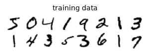
class Block(nn.Module):
"""Two convolutions with group norm, plus an additive time embedding."""
def __init__(self, c_in, c_out, c_emb):
super().__init__()
self.conv1, self.conv2 = nn.Conv2d(c_in, c_out, 3, padding=1), nn.Conv2d(c_out, c_out, 3, padding=1)
self.norm1, self.norm2 = nn.GroupNorm(8, c_out), nn.GroupNorm(8, c_out)
self.emb = nn.Linear(c_emb, c_out)
def forward(self, x, e):
h = F.silu(self.norm1(self.conv1(x))) + self.emb(e)[:, :, None, None]
return F.silu(self.norm2(self.conv2(h)))
class UNet(nn.Module):
"""Minimal three-scale U-Net: 28 -> 14 -> 7 -> 14 -> 28."""
def __init__(self, c=16, c_emb=64):
super().__init__()
self.temb = TimeEmbedding(c_emb) # same module as in section 5
self.down1, self.down2 = Block(1, c, c_emb), Block(c, 2 * c, c_emb)
self.mid = Block(2 * c, 2 * c, c_emb)
self.up2, self.up1 = Block(4 * c, c, c_emb), Block(2 * c, c, c_emb)
self.out = nn.Conv2d(c, 1, 1)
def forward(self, x, t):
e = self.temb(t, len(x))
h1 = self.down1(x, e) # 28 x 28
h2 = self.down2(F.avg_pool2d(h1, 2), e) # 14 x 14
m = self.mid(F.avg_pool2d(h2, 2), e) # 7 x 7
u = self.up2(torch.cat([F.interpolate(m, scale_factor=2), h2], dim=1), e)
u = self.up1(torch.cat([F.interpolate(u, scale_factor=2), h1], dim=1), e)
return self.out(u)
unet = UNet()
print(f"parameters: {sum(p.numel() for p in unet.parameters()):,}")parameters: 65,393STEPS, BATCH = 6000, 64
opt = torch.optim.Adam(unet.parameters(), lr=2e-3)
sched = torch.optim.lr_scheduler.CosineAnnealingLR(opt, T_max=STEPS)
mnist_losses = []
for it in range(STEPS + 1):
x0 = to_model(mnist[torch.randint(0, len(mnist), (BATCH,))]) # standardized batch
t = sample_times(BATCH)
eps = torch.randn_like(x0)
loss = ((unet(diffuse(x0, t, eps), t) - eps) ** 2).mean()
opt.zero_grad(); loss.backward(); opt.step(); sched.step()
mnist_losses.append(loss.item())
if it % 1000 == 0:
print(f"iteration {it:5d}: loss = {np.mean(mnist_losses[-200:]):.4f}")iteration 0: loss = 1.1114
iteration 1000: loss = 0.0973
iteration 2000: loss = 0.0903
iteration 3000: loss = 0.0871
iteration 4000: loss = 0.0853
iteration 5000: loss = 0.0844
iteration 6000: loss = 0.08326.1 Watching the denoising
The animation follows 16 trajectories of the reverse SDE, from pure noise to digits. Generation is coarse-to-fine, which is §1.2 read backwards: the heat equation destroys high frequencies first, so reversing it restores them last — the rough shape of each digit appears long before its strokes are sharp.
mnist_score = lambda x, t: -unet(x, t) / sigma(t)
ts_img = time_grid(300)
torch.manual_seed(3)
traj_img = reverse_sample(mnist_score, torch.randn(16, 1, 28, 28), ts_img)
digits = denoise(mnist_score, traj_img[-1], ts_img[-1])
idx = torch.linspace(0, len(ts_img) - 1, 32).long()
film = [P.image_grid(to_image(x).clamp(-1, 1), 8) for x in [*traj_img[idx], *[digits] * 6]] # hold the last frame
P.animate_images(film, figsize=(8, 2.4),
title=lambda k: f"reverse SDE, $t = {ts_img[idx[k]]:.3f}$" if k < len(idx) else "denoised")Key takeaways
- Adding Gaussian noise evolves the data distribution by a diffusion equation.
- The score is the gradient of the log density and determines the reverse drift.
- Denoising score matching learns the score by predicting noise we added ourselves.
- Exact fitting of the empirical distribution reproduces training points; generalization requires a useful model bias.
Exercises
- Take \(p_{\text{data}} = \mathcal{N}(0, s^2 I)\). Show that \(p_t = \mathcal{N}\big(0, (\alpha_t^2 s^2 + \sigma_t^2) I\big)\), so the score is linear and the reverse SDE is linear; solve it explicitly and verify numerically against
reverse_sample. - Verify Hyvärinen’s identity numerically in 1D: estimate \(\mathbb{E}_p[\tfrac12\|s_\theta\|^2 + \partial_x s_\theta]\) by Monte Carlo for a Gaussian \(p\) and compare with \(J(\theta)\) computed in closed form.
- Replace the geometric time grid by a uniform one at the same number of steps, and find where the 2-D sampler becomes unstable. Relate the threshold to \(h \lesssim \sigma_t^2\).
- Add the parameter \(\lambda\) of §2 to
reverse_sampleand compare \(\lambda = 0\) (the deterministic probability-flow ODE) with \(\lambda = 1\) on MNIST at 30, 100 and 300 steps. Which degrades faster, and why? - Add class conditioning to the MNIST model (the labels are in
train-labels-idx1-ubyte.gz) and implement classifier-free guidance by training with the label randomly dropped.
Where are we going?
Diffusion models generate by reversing a stochastic flow, with the score as the one learned ingredient. Notebook 18 closes the course’s loop in a different way: the system itself is unknown, and the control is what gets learned, from rewards.
References
The classical background
- J. Fourier, Théorie analytique de la chaleur, 1822 — the heat equation.
- A. Einstein, Über die von der molekularkinetischen Theorie der Wärme geforderte Bewegung von in ruhenden Flüssigkeiten suspendierten Teilchen, Annalen der Physik 322 (1905), 549–560.
- M. von Smoluchowski, Zur kinetischen Theorie der Brownschen Molekularbewegung und der Suspensionen, Annalen der Physik 326 (1906), 756–780.
- N. Wiener, Differential-Space, Journal of Mathematics and Physics 2 (1923), 131–174.
- A. N. Kolmogorov, Über die analytischen Methoden in der Wahrscheinlichkeitsrechnung, Mathematische Annalen 104 (1931), 415–458.
- R. P. Feynman, Space-Time Approach to Non-Relativistic Quantum Mechanics, Reviews of Modern Physics 20 (1948), 367–387.
- M. Kac, On distributions of certain Wiener functionals, Transactions of the AMS 65 (1949), 1–13.
- E. Schrödinger, Über die Umkehrung der Naturgesetze, Sitzungsberichte der Preussischen Akademie der Wissenschaften (1931), 144–153; linked English translation.
- H. Föllmer, Random fields and diffusion processes, Lecture Notes in Mathematics 1362 (1988), 101–203.
- B. D. O. Anderson, Reverse-time diffusion equation models, Stochastic Processes and their Applications 12 (1982), 313–326.
- U. G. Haussmann and E. Pardoux, Time reversal of diffusions, Annals of Probability 14 (1986), 1188–1205.
- H. Robbins, An empirical Bayes approach to statistics, Proceedings of the Third Berkeley Symposium, Vol. 1 (1956), 157–163.
- B. Efron, Tweedie’s formula and selection bias, JASA 106 (2011), 1602–1614.
Learning the score
- A. Hyvärinen, Estimation of non-normalized statistical models by score matching, JMLR 6 (2005), 695–709.
- P. Vincent, A connection between score matching and denoising autoencoders, Neural Computation 23 (2011), 1661–1674.
Diffusion models and related methods
- J. Sohl-Dickstein et al., Deep unsupervised learning using nonequilibrium thermodynamics, ICML, 2015.
- Y. Song and S. Ermon, Generative modeling by estimating gradients of the data distribution, NeurIPS, 2019.
- J. Ho, A. Jain and P. Abbeel, Denoising diffusion probabilistic models, NeurIPS, 2020.
- Y. Song et al., Score-based generative modeling through stochastic differential equations, ICLR, 2021.
- T. Karras et al., Elucidating the design space of diffusion-based generative models, NeurIPS, 2022.
- V. De Bortoli et al., Diffusion Schrödinger bridge with applications to score-based generative modeling, NeurIPS, 2021.
- Y. Lipman et al., Flow matching for generative modeling, ICLR, 2023.
- S. Lin et al., Common diffusion noise schedules and sample steps are flawed, WACV, 2024.
- R. T. Q. Chen et al., Neural ordinary differential equations, NeurIPS, 2018.
Appendix A. Feynman–Kac: the PDE / stochastic process dictionary
The bridge between the two worlds has two directions.
Forward (Kolmogorov forward / Fokker–Planck). If \(X_t\) solves \(dX_t = f(X_t,t)\,dt + g(t)\,dW_t\), then its density evolves by
\[\partial_t p_t = -\nabla\!\cdot\!\big(f\,p_t\big) + \tfrac{g(t)^2}{2}\,\Delta p_t .\]
This is a statement about densities: it pushes the law of the particles forward.
Backward (Feynman–Kac). Fix a terminal payoff \(\varphi\) and a potential \(V\). Then
\[u(x,t) = \mathbb{E}\left[\, e^{-\int_t^T V(X_s)\,ds}\,\varphi(X_T) \;\middle|\; X_t = x \right]\]
solves the linear PDE
\[\partial_t u + f\cdot\nabla u + \tfrac{g^2}{2}\Delta u = V u, \qquad u(\cdot, T) = \varphi .\]
This is a statement about observables: the value of the PDE at \((x,t)\) is an average over all trajectories started at \(x\).
Taking \(f = 0\), \(g = 1\), \(V = 0\) and reversing time (\(t \mapsto T-t\)) gives the cleanest instance of the formula, the one we care about:
\[\partial_t u = \tfrac12 \Delta u, \quad u(\cdot,0) = u_0 \qquad \Longleftrightarrow \qquad u(x,t) = \mathbb{E}\big[\,u_0(x + W_t)\,\big].\]
Solve a PDE and average over random paths are the same computation. The next cell checks this three ways: exact Gaussian convolution, finite differences, and a Monte Carlo average over Brownian paths.
# The heat equation, solved three ways at t = 0.3
x = np.linspace(-4, 4, 401)
dx = x[1] - x[0]
u0 = lambda z: np.exp(-(z + 1.5) ** 2 / 0.05) + 1.0 * ((z > 0.5) & (z < 2.0)) # bump + step
t_end = 0.3
# (a) exact: convolution with the heat kernel
K = np.exp(-(x[:, None] - x[None, :]) ** 2 / (2 * t_end)) / np.sqrt(2 * np.pi * t_end)
u_exact = K @ u0(x) * dx
# (b) explicit finite differences (stable while dt <= dx^2)
u_fd, dt = u0(x).copy(), 0.4 * dx ** 2
for _ in range(int(t_end / dt)):
u_fd[1:-1] += 0.5 * dt / dx ** 2 * (u_fd[2:] - 2 * u_fd[1:-1] + u_fd[:-2])
# (c) Feynman-Kac: simulate Brownian paths and average the initial datum at their endpoints
M, n_steps = 8000, 200
paths = np.sqrt(t_end / n_steps) * rng.standard_normal((M, n_steps))
paths = np.cumsum(paths, axis=1)
u_mc = u0(x[:, None] + paths[None, :, -1]).mean(axis=1)
fig, (axL, axR) = P.panels(2, size=(4.75, 3.6))
axL.plot(np.linspace(0, t_end, n_steps), paths[:40].T, lw=0.7, alpha=0.7, color=P.BLUE)
P.label(axL, "$t$", "$W_t$", "Brownian paths started at $x$")
P.curves(axR, x, {"$u_0$": (u0(x), {"color": P.GREY, "lw": 1.2}),
"heat kernel (exact)": (u_exact, {"color": P.BLUE, "lw": 2.5}),
"finite differences": (u_fd, {"color": P.ORANGE, "ls": "--", "lw": 1.8}),
r"Monte Carlo $\mathbb{E}[u_0(x+W_t)]$": (u_mc, {"color": P.AQUA, "ls": ":", "lw": 2.0})},
xlabel="$x$", title=f"$u(\\cdot, t)$ at $t = {t_end}$")
plt.show()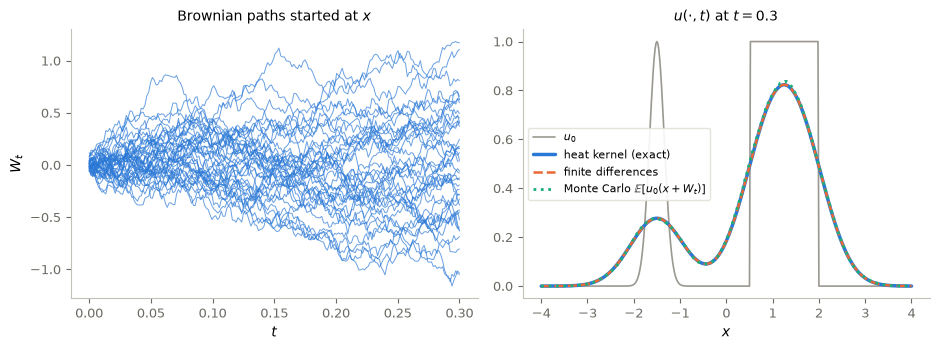
max |FD - exact| = 1.21e-04
max |Monte Carlo - exact| = 1.57e-02 (M = 8000 paths)