18 — Reinforcement Learning: From Optimal Control to Learning
Mathematical Foundations of Control and Machine Learning — Winter 2026
Central question.What remains of optimal control when the dynamics and the cost are unknown, and the only teacher is a reward signal?
Classical control steers a system whose equations of motion are known. In this notebook, we remove that assumption. Instead, we interact with the system and observe its state and reward or cost at each time step.
Table of Contents
A short history — the law of effect, Bellman at RAND, and what happened after
Two vocabularies for one problem — optimal control and reinforcement learning side by side
The Bellman equation — a contraction, and therefore an algorithm
From control to RL — Q-learning, and a note on dopamine
Exploration versus exploitation — bandits, on-policy and off-policy
Pontryagin’s maximum principle — the adjoint, direct shooting, and a trip to the Moon
Markov decision processes — the probabilistic setting
The policy gradient theorem — and REINFORCE on a problem whose answer we know
PPO — a pendulum that teaches itself to swing up
%matplotlib inlineimport numpy as npimport torchimport torch.nn as nnimport matplotlib.pyplot as pltfrom torch.distributions import Normalimport plotting as P # the course palette, the house style, and the figure helpersrng = np.random.default_rng(0)torch.manual_seed(0);
Where are we?
Recap. A feedback law \(u=F(x)\) is designed from a known model; LQR and model predictive control make that feedback optimal — for known dynamics (notebook 05). In stochastic approximation, decreasing Robbins–Monro steps tame noisy updates.
Reinforcement learning keeps the feedback structure and removes the model: the dynamics and the cost are unknown, and a policy is learned by interacting with the system. The analogy feedback ↔︎ reinforcement learning becomes the subject of this notebook, with the Bellman equation as the bridge from dynamic programming to algorithms that need no model at all.
1. A short history
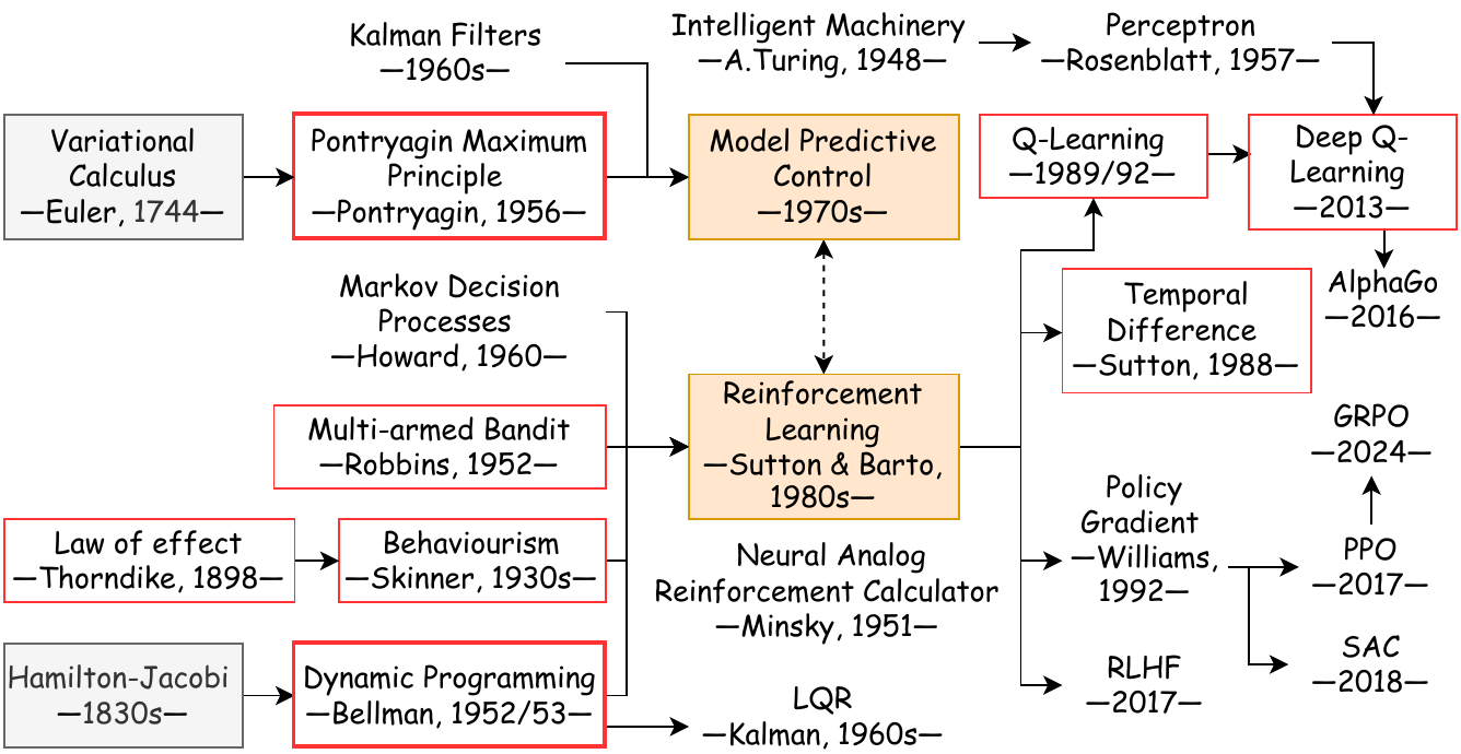
In 1898 Edward Thorndike put cats in puzzle boxes and timed how long they took to escape. The times fell with repetition, and from this he formulated the law of effect: responses followed by satisfaction become more likely, responses followed by discomfort less so. Pavlov showed around the same time that dogs can be conditioned to anticipate a stimulus, and in the 1930s B. F. Skinner made the shaping of voluntary behavior by reinforcement into an experimental science. None of this was mathematics, but it fixed the vocabulary — state, action, reward — that the mathematics would later use.
The mathematics arrived from a different direction. In the early 1950s Richard Bellman was at RAND working for the U.S. Air Force on multi-stage decisions under uncertainty: how many aircraft to commit at each stage of a mission. The method he found — solve the last stage first, then work backwards — he called dynamic programming, reportedly because “programming” sounded respectable to his sponsors and “dynamic” was impossible to use pejoratively. Out of it came the equation that carries his name, the recognition that it is a fixed-point problem, and the phrase curse of dimensionality for the reason you cannot simply solve it on a grid. By the end of the decade he had pushed it into continuous time (Appendix A), where it generalizes the Hamilton–Jacobi equation of the 1830s. In parallel, Pontryagin’s group in Moscow was deriving necessary conditions for optimal missile trajectories, and Kalman was writing down the LQR.
Learning and control met in the late 1980s. Sutton’s temporal-difference methods treated the Bellman equation as something to be satisfied on average along sampled trajectories; Watkins’ Q-learning made that idea converge to the optimal value without ever estimating the dynamics. Williams showed that one can differentiate the expected return of a stochastic policy using nothing but rollouts. Then in 1997 Schultz, Dayan and Montague reported that midbrain dopamine neurons fire in proportion to a reward-prediction error — the same quantity \(\delta_t\) that sits inside the Q-learning update. The observation suggests a connection between temporal-difference learning and biological reward signals.
What followed is mostly a story of function approximation: TD-Gammon (described in Tesauro’s 1995 article), DQN on Atari in 2015, AlphaGo in 2016, PPO in 2017, and the use of policy gradients to align language models with human preferences (Ouyang et al., 2022).
Timeline of optimal control and reinforcement learning, from Euler’s variational calculus and Thorndike’s law of effect to PPO and GRPO
2. Two vocabularies for one problem
Control theory and reinforcement learning describe the same object with different letters. The table below is a dictionary; it is worth reading once carefully, because every formula later in the notebook can be written in either column.
The last row describes the distinction used in this notebook: a known model versus learning from interaction. More generally, control can use learned models, and RL can use known ones. The sign in the second-to-last row is a convention: a reward can be defined as the negative of a cost. We will use the control letters \(x, u\) while the model is known, and switch to \(s, a\).
\(u(t,\cdot)\) supported on \(\omega \subset \Omega\)
Dynamics
\(x_{t+1} = f(x_t,u_t)\), deterministic
\(\dot x = Ax + Bu\)
\(\partial_t y = \Delta y + u \mathbf{1}_\omega\)
Objective
\(\pm 1\) at checkmate, \(0\) otherwise
\(\int_0^\infty x^\top Q x + u^\top R u \, dt\)
\(\int_0^\infty \lVert y - y^\star\rVert^2 + \lVert u\rVert^2 dt\)
Difficulty
finite but astronomically large
solved in closed form
infinite-dimensional
3. The Bellman equation
Assume bounded rewards and a finite action set, so the maxima below are attained. Fix a deterministic system and an infinite horizon with discount \(\gamma \in [0,1)\):
The third equality is the whole content of the argument: \(r(x,u_0)\) does not depend on \(u^+\), so it leaves the inner supremum, and what remains is by definition the value of the state \(f(x,u_0)\). This is the principle of optimality.
A contraction, and therefore an algorithm
Define the Bellman operator on bounded functions \(V : \mathcal{X} \to \mathbb{R}\),
Theorem.\(\mathcal{T}\) is a \(\gamma\)-contraction in the supremum norm: \(\lVert \mathcal{T}V - \mathcal{T}W \rVert_\infty \le \gamma \lVert V - W \rVert_\infty\).
Proof. Fix \(x\) and use \(\lvert \max_u F_u - \max_u G_u \rvert \le \max_u \lvert F_u - G_u \rvert\):
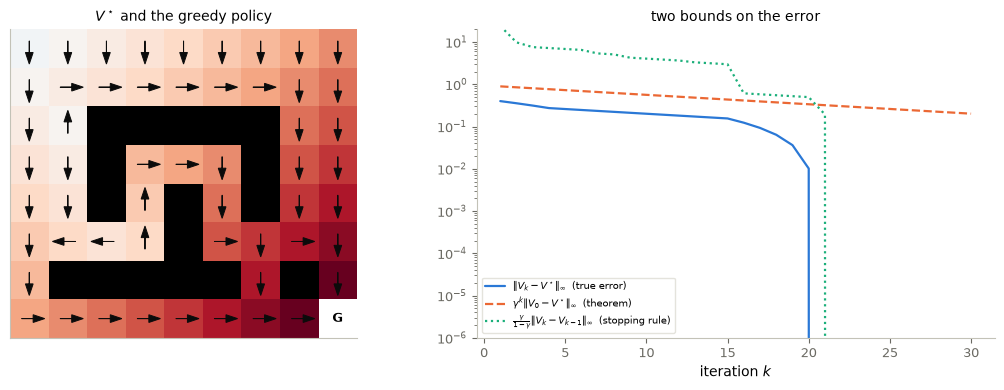
By the Banach fixed-point theorem \(V^\star\) is the unique bounded solution of \(\mathcal{T}V = V\), and value iteration\(V_{k+1} = \mathcal{T}V_k\) converges from any starting point:
The second bound is computable, so it is the one used as a stopping rule. Note what the theorem costs: one sweep evaluates every pair \((x,u)\), i.e. \(\mathcal{O}(\lvert\mathcal{X}\rvert\lvert\mathcal{U}\rvert)\) work, and it needs \(f\) and \(r\). For chess that is \(10^{43}\) states; this is Bellman’s curse of dimensionality, and it is the reason the rest of the notebook exists.
Example: Maze The environment is a grid with walls, an absorbing goal \(\mathsf{G}\) worth \(+1\). Four actions; walking into a wall leaves the state unchanged. Every other transition has reward zero, so for a nonterminal state \(V^\star(x) = \gamma^{\,d(x)-1}\), where \(d(x)\) is the length of the shortest route to the goal. The goal itself has value zero in the code. The discounting alone is what makes the agent hurry.
Code and plot. Run value iteration on a maze. Watch value propagate back from the goal.
Everything so far assumed we could evaluate\(f\) and \(r\): value iteration asks for \(r(x,u)\) and \(f(x,u)\) at every pair. Reinforcement learning drops that assumption. The agent can only act and observe:
it sees a state \(s_t\),
it chooses an action \(a_t \sim \pi(\cdot \mid s_t)\),
it receives a reward \(r_t\),
it finds itself in a new state \(s_{t+1}\).
What it collects is a stream of tuples \(\{(s_t, a_t, r_t, s_{t+1})\}_t\) and nothing else. Two families of algorithms grow out of this. Value-based methods estimate \(V\) or \(Q\) from the stream and read off a policy greedily; policy-based methods parameterize \(\pi_\theta\) and improve it directly. This section and the next do the first; §8 and §9 do the second.
Q-learning
The obstacle to using \(V\) without a model is the \(\max_u \{ r(x,u) + \gamma V(f(x,u))\}\): picking the greedy action requires knowing where each action leads. So include the first action in the value function and define the action-value function
and the greedy policy \(\pi^\star(x) \in \arg\max_u Q^\star(x,u)\) is optimal — now computable from \(Q\) alone. The corresponding operator \((\mathcal{T}Q)(x,u) := r(x,u) + \gamma\max_{u'}Q(f(x,u),u')\) is again a \(\gamma\)-contraction, by the same two lines as before, so \(Q^\star\) exists and is unique.
This is still a model-based identity. The step that makes it an algorithm is to stop solving the equation and start correcting towards it, one observed transition at a time. Given a sample \((s_t, a_t, r_t, s_{t+1})\), form the temporal-difference error
\[\delta_t := \underbrace{r_t + \gamma \max_{a'} Q(s_{t+1},a')}_{\text{what the data say}} \;-\; \underbrace{Q(s_t,a_t)}_{\text{what we believed}},
\qquad Q(s_t,a_t) \leftarrow Q(s_t,a_t) + \alpha\,\delta_t .\]
\(\delta_t\) is an unbiased sample of the Bellman residual at \((s_t,a_t)\), so the update is a stochastic approximation to \(Q \leftarrow \mathcal{T}Q\). Watkins and Dayan (1992) proved it converges to \(Q^\star\) with probability one, provided every state–action pair is visited infinitely often and, for each state–action pair, the step sizes across its visits satisfy the Robbins–Monro conditions \(\sum_j \alpha_j = \infty\), \(\sum_j \alpha_j^2 < \infty\). The first condition is not a technicality: it is the whole subject of §5.
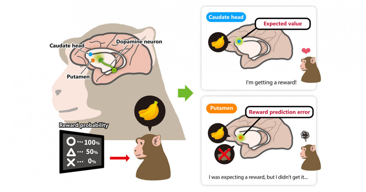
An aside on dopamine. In 1997 Schultz, Dayan and Montague recorded midbrain dopamine neurons in monkeys. The neurons fired when an unexpected reward arrived; after a predictive cue was learned, they fired at the cue instead; and when an expected reward failed to appear, their activity dipped below baseline at exactly the moment it was due. That is the sign pattern of \(\delta_t\), not of reward. The reward-prediction-error hypothesis — that dopamine broadcasts \(\delta_t\) — remains one of the closest contacts between a machine-learning algorithm and a measured biological signal.
Dopamine neurons in the macaque basal ganglia: expected value in the caudate head, reward-prediction error in the putamen
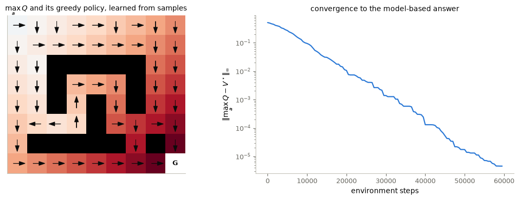
Below, the same grid world as §3, but the agent is given only NEXT and R as an oracle it may query at its current state: it never reads them as tables, never sweeps over the state space, and never sees a transition it did not itself take.
Code and plot. Learn the same maze from sampled transitions and compare the error with value iteration.
start = np.flatnonzero(~term) # episodes begin anywhere, so every pair is reachableQ, s, err_q = np.ones((len(free), 4)), rng.choice(start), [] # optimistic init: unseen actions look goodfor t inrange(60_000): a = rng.integers(4) if rng.random() <0.1else Q[s].argmax() # epsilon-greedy s2, r = NEXT[s, a], R[s, a] # the environment answers delta = r + GAMMA * (0.0if term[s2] else Q[s2].max()) - Q[s, a] # temporal-difference error Q[s, a] +=0.2* delta s = rng.choice(start) if term[s2] else s2if t %500==0: err_q.append(np.abs(np.where(term, 0, Q.max(1)) - V_star).max())pi_q = Q.argmax(1)print(f"||max_a Q - V*||_inf = {err_q[-1]:.2e}")print(f"sub-optimality of greedy pi = {np.abs(V_star - (R + GAMMA * V_star[NEXT])[np.arange(len(free)), pi_q])[~term].max():.2e}")
||max_a Q - V*||_inf        = 4.55e-06
sub-optimality of greedy pi = 0.00e+00
fig, (a0, a1) = P.panels(2, size=(5.5, 4))draw_values(a0, np.where(term, 0, Q.max(1)), pi_q, title=r"$\max_a Q$ and its greedy policy, learned from samples")P.curves(a1, np.arange(len(err_q)) *500, err_q, log="y", xlabel="environment steps", ylabel=r"$\|\max_a Q - V^\star\|_\infty$", title="convergence to the model-based answer")plt.show()
The learned value field is indistinguishable from the one value iteration computed with full knowledge of \(f\) and \(r\), and the induced policy is exactly optimal (where the arrows differ, the two actions have equal value). The price is on the horizontal axis. Value iteration settled in a couple of dozen sweeps; Q-learning needed tens of thousands of steps of interaction to reach the same answer, and it had to walk to every state it wanted to learn about. In dynamic programming the currency is computation; in reinforcement learning it is experience.
Two details in the code carry weight. Q = np.ones(...) is optimistic initialization: since true values are below \(1\), any action never tried looks better than one already tried, and the agent sweeps its options without being told to. Episodes restart from a uniformly random nonterminal state, and \(\varepsilon\)-greedy actions provide exploration. The fixed step size \(0.2\) keeps this deterministic example short; it does not satisfy the diminishing-step-size conditions of the general convergence theorem. Without exploration, zero initialization and ties broken by index can leave the agent repeatedly choosing up against a wall.
5. Exploration versus exploitation
Watkins’ theorem needs every state–action pair visited infinitely often, but the policy we are learning is greedy, and a greedy policy visits what it already likes. The standard compromise is the \(\varepsilon\)-greedy rule: behave greedily, except that with probability \(\varepsilon\) act at random,
\[a_t \sim \begin{cases}\arg\max_{a} Q(s_t,a), & \text{with probability } 1-\varepsilon,\\[2pt]
\mathrm{Uniform}(\mathcal{A}), & \text{with probability } \varepsilon.\end{cases}\]
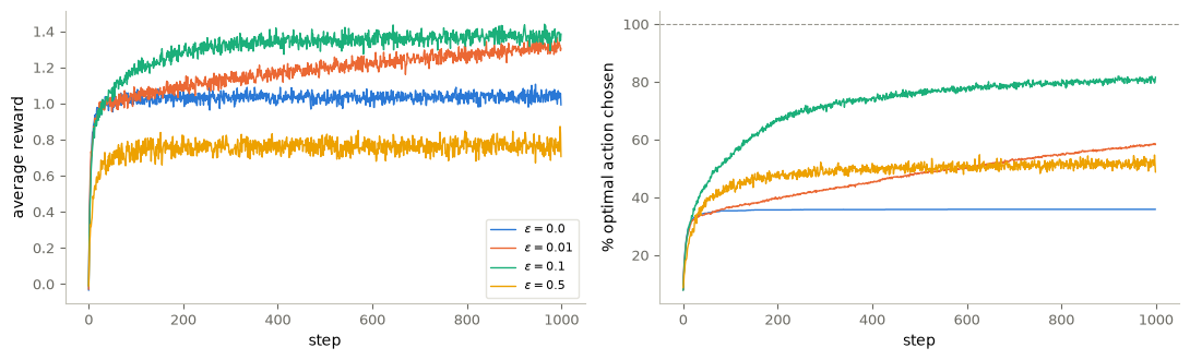
Both extremes fail. At \(\varepsilon = 0\) the agent never revises a bad early estimate; at \(\varepsilon = 1\) it keeps choosing random actions even after it has learned which actions are better. The cleanest place to see the trade-off is the multi-armed bandit of Robbins (1952): a single state, \(K\) actions, and reward \(r(a) \sim \mathcal{N}(\mu_a, 1)\). Here the best expected reward per pull is \(\max_a \mu_a\) and \(Q(a) \to \mu_a\) is just an average of samples, so nothing but the exploration question remains.
Code and plot. Compare reward and optimal-action frequency for several exploration rates.
K, RUNS, STEPS =10, 2000, 1000mu = rng.standard_normal((RUNS, K)) # one bandit instance per runbest, ix = mu.argmax(1), np.arange(RUNS)def run_eps(eps): Q, N, out = np.zeros((RUNS, K)), np.zeros((RUNS, K)), np.zeros((STEPS, 2))for t inrange(STEPS): a = np.where(rng.random(RUNS) < eps, rng.integers(K, size=RUNS), Q.argmax(1)) r = mu[ix, a] + rng.standard_normal(RUNS) N[ix, a] +=1 Q[ix, a] += (r - Q[ix, a]) / N[ix, a] # running mean = step size 1/N out[t] = r.mean(), (a == best).mean()return outfig, (a0, a1) = P.panels(2, size=(5.5, 3.4))for eps in [0.0, 0.01, 0.1, 0.5]: out = run_eps(eps) a0.plot(out[:, 0], lw=1, label=rf"$\varepsilon = {eps}$"); a1.plot(100* out[:, 1], lw=1)a1.axhline(100, color=P.GREY, lw=0.8, ls="--")P.label(a0, "step", "average reward")P.label(a1, "step", "% optimal action chosen")plt.show()
Pure greed (\(\varepsilon = 0\)) rises fastest for the first few pulls and then stops: it commits to whichever arm happened to pay first, and after a thousand steps is still choosing the best arm only about a third of the time. High exploration (\(\varepsilon = 0.5\)) does the opposite — it finds the best arm reliably and then throws away half of its pulls on arms it knows are worse, so it earns the least of the four. The two panels rank these two differently, which is the point: knowing which arm is best and actually playing it are separate achievements, and \(\varepsilon\) decides how much of one you trade for the other.
The useful values are small and positive, and the right one depends on the horizon: on a longer run \(\varepsilon = 0.01\) eventually overtakes \(\varepsilon = 0.1\), which is why \(\varepsilon\) is normally annealed towards zero. Modern alternatives replace the uniform noise with something directed: optimism (UCB), posterior sampling (Thompson), or an entropy bonus in the objective itself, which is the route PPO takes in §9.
On-policy and off-policy
There are two policies in the room. The behavior policy\(\mu\) generates the data; the target policy\(\pi\) is the one being improved. Q-learning’s update uses \(\max_{a'} Q(s_{t+1},a')\) — the value of the greedy action — while the data was gathered by an \(\varepsilon\)-greedy walk. Target \(\neq\) behavior, so Q-learning is off-policy. Replacing that \(\max\) by \(Q(s_{t+1}, a_{t+1})\), the action actually taken next, gives SARSA, which is on-policy.
On-policy (\(\mu = \pi\))
Off-policy (\(\mu \neq \pi\))
Examples
SARSA, REINFORCE, A2C, TRPO, PPO
Q-learning, DQN, DDPG, TD3, SAC
Data
usually fresh rollouts; PPO reuses a batch for several epochs
may be kept in a replay buffer and reused
Sample efficiency
low
high
Stability
more stable, simpler theory
can diverge — the deadly triad
The deadly triad (Sutton and Barto, 2018): bootstrapping, function approximation and off-policy data are each harmless alone, and jointly can make the iteration diverge — the composition of a \(\gamma\)-contraction with a projection onto the span of the features need not be a contraction in any norm. DQN’s target networks and replay buffers exist to make the composition behave.
6. Pontryagin’s maximum principle
Dynamic programming is not the only route to optimality, and historically it was not the only one being built. While Bellman was at RAND, Lev Pontryagin’s group in Moscow was working on trajectory optimization for ballistic missiles, and arrived at necessary conditions of a completely different shape: no value function on the state space, just two coupled ODEs along a single trajectory.
Introduce the Hamiltonian\(H(x,u,p) := \ell(x,u) + p^\top f(x,u)\).
Theorem (Pontryagin et al., 1962; normal, smooth case). If \((x^\star, u^\star)\) is optimal, there is an adjoint (costate) \(p : [0,T] \to \mathbb{R}^n\) with
Choosing \(p\) to annihilate the \(\delta x\) terms gives the adjoint equation and its terminal condition, and what is left multiplying \(\delta u\) is the gradient: \(\nabla_{u(t)}J = \nabla_u \ell + (\nabla_u f)^\top p_t\). The multiplier is a sensitivity — when the value function is differentiable, \(p_t = \nabla_x V(t, x^\star_t)\), which is how the two theories touch. Here \(V\) solves the Hamilton–Jacobi–Bellman equation, the continuous-time Bellman equation derived in Appendix A, and the two routes compare as follows:
HJB
PMP
Unknown
\(V(t,x)\) on \([0,T]\times\mathcal{X}\)
\((x^\star_t, p_t)\) on \([0,T]\)
Equation
a PDE on the state space
ODEs along one trajectory
Yields
a feedback law \(u^\star(x)\) (closed loop)
a control signal \(u^\star(t)\) (open loop)
Conditions
necessary and sufficient
necessary only
Cost
a state-space grid grows exponentially with dimension
trajectory computation grows with state dimension and horizon
The last row is why PMP survives in high dimensions and HJB does not, and it is the reason trajectory optimization and model predictive control are written this way.
Direct shooting is reverse-mode autodiff
Discretise with Euler, \(x_{t+1} = x_t + \Delta t\, f(x_t,u_t)\), and repeat the Lagrangian argument with multipliers \(\hat p_{t+1}\). What comes out is a backward sweep and a gradient:
This is exactly what reverse-mode automatic differentiation does when you backpropagate through the Euler unroll — the adjoint \(\hat p_t\) is the gradient of the loss with respect to \(x_t\), which is the quantity backward() propagates. So direct shooting is three lines:
forward-simulate \(x_0,\dots,x_N\) from the current \(u\);
call J.backward(), which runs the adjoint sweep;
step \(u \leftarrow u - \eta\,\nabla_u J\), and repeat.
With \(\theta\) in place of \(u\) and a data-fitting loss in place of \(\int\ell\), these three lines are exactly the training loop of a neural ODE; that is all a neural ODE is.
Optional example: a trip to the Moon
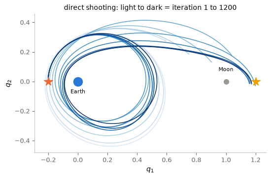
A simplified planar gravitational model with the Earth at the origin and the Moon fixed at \((1,0)\), state \(x = (q, v) \in \mathbb{R}^4\), control the thrust acceleration \(u \in \mathbb{R}^2\):
\[\dot q = v, \qquad \dot v = -\mu_E\frac{q - q_E}{\lVert q-q_E\rVert^3} - \mu_M\frac{q-q_M}{\lVert q - q_M\rVert^3} + u .\]
The spacecraft starts in a low Earth orbit whose natural apoapsis falls well short of the Moon, so it cannot coast there — the optimizer must apply thrust. The cost is a quadratic control-effort surrogate plus a terminal penalty for missing the target lunar orbit, with one waypoint term to break the symmetry between going the long way round and the short way:
traj = snaps[-1][::6]def bodies(ax): # Earth and Moon, fixed in the frame ax.plot(*qE, "o", ms=13, color=P.BLUE); ax.plot(*qM, "o", ms=7, color=P.GREY)P.animate_trajectory(traj, decorate=bodies, figsize=(5.0, 4.2), title=lambda k: f"$t = {k *6* dt:.2f}$")
7. Markov decision processes
Everything so far was deterministic: \(f\) was a map, and the only randomness was the agent’s own exploration. Real environments are noisy, and the standard object is the Markov decision process, a tuple \(\mathcal{M} = (\mathcal{S}, \mathcal{A}, P, r, \gamma)\):
a measurable state space \((\mathcal{S}, \mathcal{F}_\mathcal{S})\) and action space \((\mathcal{A}, \mathcal{F}_\mathcal{A})\);
a transition kernel\(P : \mathcal{S}\times\mathcal{A} \to \mathcal{P}(\mathcal{S})\), where \(P(\cdot\mid s,a)\) is a probability measure and \((s,a)\mapsto P(B\mid s,a)\) is measurable for every \(B \in \mathcal{F}_\mathcal{S}\): \[P(B \mid s,a) = \mathbb{P}\big(S_{t+1}\in B \mid S_t = s,\, A_t = a\big);\]
The defining assumption is the Markov property: for every measurable \(B \subseteq \mathcal{S}\),
\[\mathbb{P}\big(S_{t+1} \in B \mid S_0,A_0,\dots,S_t,A_t\big) = P(B\mid S_t,A_t),\]
the future depends on the past only through the present state and action. A policy is a kernel \(\pi : \mathcal{S}\to\mathcal{P}(\mathcal{A})\), and the value functions are
The contraction proof is unchanged — an integral against a probability measure is an average, and averaging is a non-expansion in \(\lVert\cdot\rVert_\infty\) — so value iteration still converges at rate \(\gamma\).
Note that a stochastic policy is now a first-class object rather than an exploration hack. For an MDP with full state observation under standard assumptions, such as finite state and action spaces with bounded rewards, there is a deterministic optimal policy, so the randomness buys nothing at the optimum — but it is what makes \(\pi_\theta\) differentiable, which is the whole of the next section.
8. The policy gradient theorem
Value-based methods detour through \(Q\) and then take an \(\arg\max\), which is awkward when \(\mathcal{A}\) is continuous: the greedy step becomes an optimization problem of its own, solved at every time step. Policy-based methods remove the detour. Parametrise \(\pi_\theta(a\mid s)\) and do gradient ascent on
The difficulty is that \(\theta\) changes the distribution being averaged over, not the integrand, and we cannot differentiate \(P\) because we do not know it.
Proof sketch.(1) The score trick. Assume the policy is differentiable and the derivative can be passed under the expectation (bounded returns alone do not guarantee this). Then \(\nabla_\theta p_\theta = p_\theta \nabla_\theta \log p_\theta\):
Taking logs of the factorisation, \(\nu\) and \(P\) are free of \(\theta\) and drop out: \(\nabla_\theta \log p_\theta(\tau) = \sum_{t\ge0}\nabla_\theta\log\pi_\theta(A_t\mid S_t)\). The unknown dynamics have disappeared — this is the step that makes the whole method possible.
(2) The score is centered. For every fixed \(s\), \(\mathbb{E}_{a\sim\pi_\theta}[\nabla_\theta\log\pi_\theta(a\mid s)] = \nabla_\theta\!\int \pi_\theta(a\mid s)\,da = \nabla_\theta 1 = 0.\)
(3) Causality. Let \(\mathcal{F}_t = \sigma(S_0,A_0,R_1,\dots,R_t,S_t)\), the history before\(A_t\). For \(k < t\) the reward \(R_{k+1}\) is \(\mathcal{F}_t\)-measurable, so by the tower property and step (2),
An action cannot affect a reward that has already been paid, so only \(k\ge t\) survives.
(4) Markov. With \(\mathcal{G}_t = \sigma(\mathcal{F}_t, A_t)\), the law of the future given \(\mathcal{G}_t\) depends on the history only through \((S_t,A_t)\), hence \(\mathbb{E}[\sum_{k\ge t}\gamma^{k-t}R_{k+1}\mid\mathcal{G}_t] = Q^{\pi_\theta}(S_t,A_t)\).
(5) Assemble. Factor \(\gamma^k = \gamma^t\gamma^{k-t}\) and apply the tower with \(\mathcal{G}_t\), pulling out the \(\mathcal{G}_t\)-measurable score. Summing over \(t\) gives the theorem. \(\square\)
REINFORCE
\(Q^{\pi_\theta}\) is unknown, but by definition it is the conditional mean of the realized return, so along a sampled rollout \(G_t = \sum_{k\ge0}\gamma^k r_{t+k+1}\) is an unbiased estimate of it. Substituting gives Williams’ REINFORCE (1992):
roll out \(\{s_t,a_t,r_{t+1}\}_{t=0}^{T}\) with \(a_t\sim\pi_\theta(\cdot\mid s_t)\);
Unbiased, and badly behaved: \(G_t\) sums an entire trajectory, so its variance grows with the horizon. The standard repair is a baseline — replace \(G_t\) by \(G_t - b(s_t)\) for any function of the state alone. Step (2) of the proof shows this changes nothing in expectation, while it can reduce the variance a great deal. Below we center and scale the sampled returns within a batch for a compact demonstration. Because the batch mean includes each sample’s own return, this practical estimator differs from the exactly unbiased state-baseline estimator above. The code also omits the outer \(\gamma^t\) weight, so it illustrates a common policy-gradient surrogate rather than the exact discounted-gradient formula.
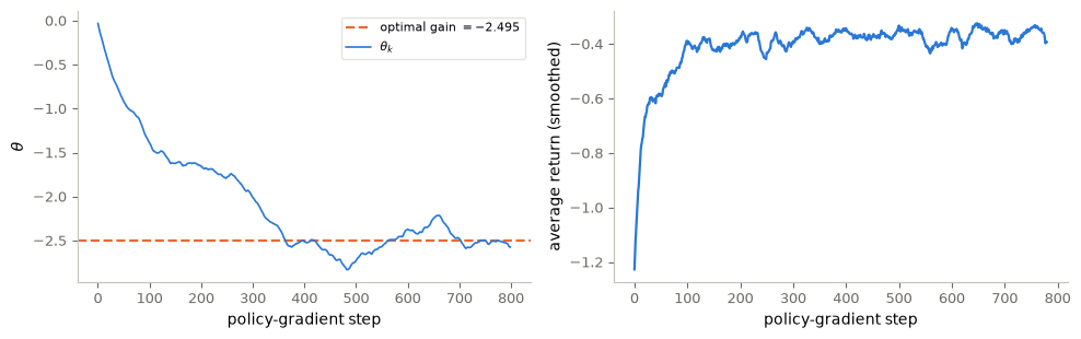
Example (scalar LQ, a test with a known answer). Take \(\dot x = u\), Euler-stepped with \(\Delta t = 0.1\), running cost \((x^2 + 0.1\,u^2)\,\Delta t\) and discount \(\gamma = e^{-\rho\Delta t}\), \(\rho = 0.5\). The value function is \(V(x) = p\,x^2\), where \(p\) is the fixed point of the Bellman backup of §3,
and the optimal feedback is \(u = \theta^\star x\) with \(\theta^\star\) the minimizer at the fixed point (Appendix A: what it becomes as \(\Delta t \to 0\)). Take the policy \(\pi_\theta(u \mid x) = \mathcal{N}(\theta x, \sigma^2)\). REINFORCE sees only states, actions and costs, yet \(\theta\) should approach \(\theta^\star\).
Code and plot. Learn a scalar feedback gain and compare it with a gain computed from the known model.
A_LQ, B_LQ, Q_LQ, R_LQ, RHO =0.0, 1.0, 1.0, 0.1, 0.5def gain(p, dt): # the minimiser, u = gain * x g = np.exp(-RHO * dt)return-g * p * B_LQ * (1+ A_LQ * dt) / (R_LQ + g * p * B_LQ **2* dt)def p_discrete(dt): # fixed point of the Delta-t backup g, p = np.exp(-RHO * dt), 0.0for _ inrange(int(60/ dt)): k = gain(p, dt) p = (Q_LQ + R_LQ * k **2) * dt + g * p * (1+ (A_LQ + B_LQ * k) * dt) **2return pDT, T_EP, SIGMA, BATCH =0.1, 100, 0.3, 32GAMMA_C =float(np.exp(-RHO * DT))theta_star = gain(p_discrete(DT), DT) # the optimal gain of the discretised problemtorch.set_default_dtype(torch.float32)theta = torch.zeros(1, requires_grad=True)opt = torch.optim.Adam([theta], lr=3e-2)theta_hist, ret_hist = [], []for ep inrange(800): x, logp, rew = torch.randn(BATCH), [], []for t inrange(T_EP): # one batch of rollouts d = Normal(theta * x, SIGMA) u = d.sample() logp.append(d.log_prob(u)); rew.append(-(Q_LQ * x **2+ R_LQ * u **2) * DT) x = x + DT * u logp, rew = torch.stack(logp), torch.stack(rew) G, g = torch.zeros_like(rew), 0.0for t inreversed(range(T_EP)): # returns-to-go g = rew[t] + GAMMA_C * g; G[t] = g adv = (G - G.mean(1, keepdim=True)) / (G.std() +1e-8) # baseline, then rescale loss =-(logp * adv).sum(0).mean() opt.zero_grad(); loss.backward(); opt.step() theta_hist.append(theta.item()); ret_hist.append(G[0].mean().item())print(f"REINFORCE theta = {theta.item():.4f} optimal gain = {theta_star:.4f}")
Optional training extension. REINFORCE has two defects. Its gradient estimate is noisy, and each batch of data can be used for exactly one step — after the update the data is off-policy and the estimator is no longer valid. PPO (Schulman et al., 2017) repairs both, and in doing so became the default algorithm for continuous control and, later, for aligning language models.
A critic, to reduce variance. Train a value network \(V_\phi\) alongside the policy. From the temporal-difference residuals \(\delta_t = r_{t+1} + \gamma V_\phi(s_{t+1}) - V_\phi(s_t)\), form the generalized advantage estimate (Schulman et al., 2016)
which interpolates between \(\lambda = 0\) (one-step TD: low variance, biased by the critic’s error) and \(\lambda = 1\) (the Monte-Carlo return minus a baseline: unbiased, high variance). It answers “how much better was \(a_t\) than what the critic expected of this state?”. The critic is fitted to its own targets, \(L^{\text{VF}} = \mathbb{E}_t[(V_\phi(s_t) - R_t)^2]\) with \(R_t = A_t + V_\phi(s_t)\).
A clip, to reuse the batch. Importance sampling lets a batch drawn under \(\pi_{\theta_{\text{old}}}\) estimate the objective at a nearby \(\theta\), through the ratio \(\varrho_t(\theta) = \pi_\theta(a_t\mid s_t)/\pi_{\theta_{\text{old}}}(a_t\mid s_t)\) — but only while the two policies are close, since the variance of the estimate blows up with the ratio. PPO discourages large changes by clipping the policy ratio in a surrogate objective:
If \(A_t > 0\) the objective stops rewarding increases in \(\varrho_t\) beyond \(1+\epsilon\); if \(A_t<0\) it stops rewarding decreases below \(1-\epsilon\). For these favorable changes beyond the clip, the clipped contribution has zero gradient. The \(\min\) retains penalties for changes that worsen the sampled advantage. This permits several optimization epochs on one rollout batch, but clipping is a heuristic: it does not impose a hard bound on the policy change or guarantee improved return.
An entropy bonus, to keep exploring.\(\mathcal{H}[\pi_\theta] = -\mathbb{E}_{a\sim\pi_\theta}[\log \pi_\theta(a\mid s)]\) rewards keeping the action distribution broad. Unlike \(\varepsilon\)-greedy, it is part of the objective and differentiable, so the policy decides for itself how much noise to keep. The full loss is
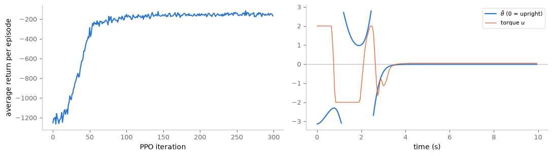
This is a pendulum swing-up task, a problem that MPC solves when the dynamics are known. Here the agent gets \((\cos\theta,\sin\theta,\dot\theta/8)\), a torque bounded by \(\lvert u \rvert \le 2\) — too weak to lift the pendulum directly, so it must pump energy by rocking — and the reward
Other things worth a notebook of their own.Model-based RL learns \(f\) and \(r\) from data and then plans against them — drop a neural ODE into the place where MPC expects its model, and that is the whole idea. Inverse RL infers \(r\) from expert demonstrations; imitation learning skips \(r\) and copies the expert directly. Multi-agent RL puts several learners in one environment, where the stationarity the Markov property assumes is gone. Meta-RL learns across a family of environments.
The difficulties, stated plainly.
Exploration. The \(\varepsilon\)-greedy rule of §5 is a placeholder. In a long-horizon task with a single reward at the end, random actions essentially never find it.
Credit assignment. When the reward arrives a thousand steps after the decision that caused it, \(\gamma^t\) has already made the signal negligible.
Sample efficiency. The pendulum above cost millions of steps for a problem a controls engineer solves with a pen. This is tolerable in a simulator and often prohibitive on hardware.
Reward design and reward hacking. The agent optimizes what you wrote, not what you meant. The \(0.001\,u^2\) term in the pendulum reward is there to stop it chattering the torque; remove it and watch.
Instability. Seeds, reward scaling and learning rates change results more than algorithmic choices do. Published comparisons are frequently within seed noise.
MPC or RL? It is not a competition so much as a question of where you want to spend. MPC needs a model and online computation, and gives constraint satisfaction, stability certificates and immediate adaptation to a new cost. RL needs data and offline computation, and gives a policy that is cheap to evaluate and does not care how nasty the dynamics are. The interesting work is in between: data-driven MPC, which learns the model and keeps the guarantees, and model-based RL, which plans against a learned model. The practical question is how much useful information each interaction provides.
And the mathematics we only touched. Viscosity solutions of the HJB equation (Appendix A); convergence rates of stochastic approximation; the geometry behind the trust region in PPO (natural gradients and TRPO); continuous-time RL, where the Bellman backup becomes an SDE problem and recent work is actively reopening the question; and the fact that score-based diffusion sampling is itself a stochastic optimal control problem, whose optimal control turns out to be the score.
Key takeaways
The Bellman equation expresses a decision as immediate reward plus future value.
Value iteration uses a model; Q-learning estimates action values from observed transitions.
Exploration provides information about actions the current policy would otherwise avoid.
Policy gradients improve a parameterized policy using sampled returns; PPO adds a critic and a clipped surrogate.
Exercises
Discounting. Run value iteration with GAMMA = 0.5 and GAMMA = 0.99. Compare how far the goal’s value propagates through the maze.
Exploration. Compare the bandit curves for eps = 0, 0.01, and 0.1. Which rule earns more reward early and late?
Learning from samples. Change the Q-learning step size from 0.2 to 0.05. Plot the error against environment steps and explain the trade-off.
Where are we going?
This notebook closes the loop of the course: the course began by asking what it means to act on a dynamical system, and here the action itself is learned from rewards. Notebook 19 collects the three threads of the course — adjoints and gradients, gradient dynamics, controllability and representation — and classifies every control ↔︎ machine-learning connection by its kind and its scope.
Appendix A. Continuous time: the Hamilton–Jacobi–Bellman equation
The Bellman equation of §3 describes a sequence of decisions at discrete times. A mechanical system does not wait for them, and the equation has a continuous-time limit.
Derivation. Take a step of length \(\Delta t\). The reward accrued is \(r(x,u)\Delta t\), the discount applied is \(\gamma^{\Delta t}\), and the state moves to \(x + f(x,u)\Delta t\). The discrete Bellman equation reads
Expand both the discount and the value to first order, \(\gamma^{\Delta t} = 1 + \ln(\gamma)\Delta t + o(\Delta t)\) and \(V(x + f\Delta t) = V(x) + \nabla V(x)^\top f \Delta t + o(\Delta t)\):
Writing \(\gamma = e^{-\rho}\) puts it in its usual form, \(\rho V = \max_u \{ r + \nabla V^\top f\}\). This is the Hamilton–Jacobi–Bellman equation: a first-order, fully nonlinear PDE on the state space. Its solutions are generally not differentiable and the right notion is a viscosity solution (Crandall and Lions, 1983), for which existence and uniqueness can be established under suitable assumptions.
A check on the scalar problem of §8. Take \(\dot x = ax + bu\) with cost \(q x^2 + \mathsf{r}\,u^2\); in the cost convention the \(\max\) becomes a \(\min\). Try \(V(x) = p\,x^2\). The minimizer is \(u = -(pb/\mathsf{r})\,x\), and the HJB equation collapses to the algebraic Riccati equation
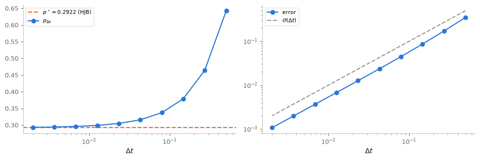
Below, its positive root is compared with the fixed point p_discrete(\(\Delta t\)) of the discrete backup of §8, with \(a = 0\), \(b = 1\), \(q = 1\), \(\mathsf{r} = 0.1\), \(\rho = 0.5\) as there.
continuous-time optimal feedback:  u = -2.9221 x
its Delta t = 0.1 counterpart:     u = -2.4951 x
The error is first order in \(\Delta t\), which is what an Euler discretization of the dynamics together with a first-order expansion of \(\gamma^{\Delta t}\) should give.
Keep the second number in mind. An agent that acts every \(\Delta t = 0.1\) is solving the discrete problem, not the continuous one, so \(-2.4951\) — not \(-2.9221\) — is the gain it should find. That is the target §8 hands to REINFORCE, an algorithm that knows neither \(a\), \(b\), \(q\) nor \(\mathsf{r}\).