%matplotlib inline
import pathlib, urllib.request
import numpy as np
import torch
import torch.nn as nn
import matplotlib.pyplot as plt
import plotting as P           # the course palette, the house style, and the figure helpers

torch.manual_seed(0)
rng = np.random.default_rng(15);15 — Transformers: Attention and Token Dynamics
Mathematical Foundations of Control and Machine Learning — Winter 2026
Central question. What happens when the moving points interact, as tokens do in a transformer — and what can be built, and what can be proved, about where they go?
The transformer (Vaswani et al., 2017) replaced recurrence by a single operation: self-attention, a learned, data-dependent weighted average over a sequence. This notebook first builds the architecture from the equations up — in about a hundred lines — and trains a miniature BERT on Shakespeare. It then strips the model down to pure hardmax attention, where the tokens become an interacting-particle system: leaders, shrinking convex hulls and a clustering theorem, proved and observed.
Table of Contents
- Self-attention — queries, keys, values, and the kernel view
- Why \(1/\sqrt{d_a}\) — keeping the softmax awake
- Multi-head attention — several low-rank views of the same sequence
- Positional encoding — attention is a set operation; order has to be injected
- The transformer block — residual stream, LayerNorm, token-wise MLP
- Masked language modeling — a character-level BERT on Tiny Shakespeare, and generation
- Tokens as interacting particles — hardmax attention and the normalized update
- Two facts, with proofs — the hull shrinks; leaders stay put
- The clustering theorem and what it assumes
- Laboratory: toy tokens, forty layers and beyond
- Softmax at low temperature, and ties
- Sentiment analysis and prompt engineering
- Modern self-attention — what changes at \(10^{11}\) parameters
- Control ↔︎ ML
- Exercises
Notation. Tokens \(z_i\in\mathbb R^d\), \(i=1,\dots,n\), configuration \(Z=(z_1,\dots,z_n)\), layer index \(k\), depth \(K\). Local overloads: \(n\) is the number of tokens (not a state dimension), \(A\) is the attention matrix (not a system matrix), and \(\alpha\) is the attention step size (not a strong-convexity constant or a control-cost weight).
Where are we?
Recap. A residual layer \(x_{k+1}=x_k+hf(x_k,\theta_k)\) moves each data point by a field that depends on that point only (notebook 13). One control can steer many points, and a fixed half-space readout turns final positions into labels.
In a transformer the points, called tokens, still move layer by layer, but each one moves according to the positions of all the others. The network becomes a system of interacting particles. Sections 1–6 build and train the real architecture; sections 7–12 study the simplest mathematical model of its interaction, hardmax self-attention (Alcalde, Fantuzzi and Zuazua, 2025), prove two of its basic properties, transcribe the clustering theorem, and observe the dynamics on toy tokens.
1. Self-attention
Take \(n\) input vectors \(x_i \in \mathbb{R}^{d_m}\), stacked as rows of \(X \in \mathbb{R}^{n \times d_m}\). Three learned projections turn each token into a query, a key and a value, \[ Q_i = W_Q^\top x_i, \qquad K_j = W_K^\top x_j, \qquad V_j = W_V^\top x_j, \] with \(W_Q, W_K \in \mathbb{R}^{d_m \times d_a}\) and \(W_V \in \mathbb{R}^{d_m \times d_v}\); in matrix form \(Q = X W_Q\), \(K = X W_K\), \(V = X W_V\). Token \(i\) asks a question with \(Q_i\), token \(j\) advertises what it is with \(K_j\), and the match is measured by an inner product. The attention weight from \(i\) to \(j\) is \[ \alpha_{ij} = \operatorname{softmax}_j\!\left(\frac{\langle Q_i, K_j\rangle}{\sqrt{d_a}}\right) = \frac{\exp\!\big(\langle Q_i, K_j\rangle / \sqrt{d_a}\big)} {\sum_{k} \exp\!\big(\langle Q_i, K_k\rangle / \sqrt{d_a}\big)}, \qquad\qquad \operatorname{Attn}(x_i, X) = \sum_j \alpha_{ij} V_j . \]
Three observations set the tone for everything that follows.
(i) It is an average. Each row \(\alpha_i\) lives in the probability simplex, so the output is a convex combination of the values. Attention interpolates between tokens; it never leaves the convex hull of \(V\).
(ii) It is a kernel method. Writing \(\kappa(x_i, x_j) = \exp\big(\langle Q_i, K_j\rangle/\sqrt{d_a}\big)\), \[ \operatorname{Attn}(x_i, X) = \frac{\sum_j \kappa(x_i, x_j)\, V_j}{\sum_k \kappa(x_i, x_k)}, \] which is exactly the classical Nadaraya–Watson kernel regression estimator with a kernel that is learned.
(iii) It costs \(\mathcal{O}(n^2)\). Every pair \((i,j)\) is scored, so \(n^2 d_a\) operations and — unless one is careful — an \(n \times n\) matrix in memory. This single quadratic is the reason for much of modern architecture research (§13).
Code and plot. Compute attention in a few lines, check the row sums, and plot the attention matrix.
n, d_model, d_attn, d_value = 15, 5, 4, 16          # tokens, d_m, d_a, d_v
X = torch.randn(n, d_model)
Wq, Wk, Wv = torch.randn(d_model, d_attn), torch.randn(d_model, d_attn), torch.randn(d_model, d_value)

def self_attention(X, Wq, Wk, Wv):
    Q, K, V = X @ Wq, X @ Wk, X @ Wv                # [n,da], [n,da], [n,dv]
    scores = Q @ K.T / Q.shape[-1] ** 0.5           # einsum('il,jl->ij', Q, K)   [n,n]
    alpha = scores.softmax(dim=1)                   # row-stochastic              [n,n]
    return alpha @ V, alpha                         # einsum('ij,jd->id', ...)    [n,dv]

Y, alpha = self_attention(X, Wq, Wk, Wv)
print("Y:", tuple(Y.shape), " alpha:", tuple(alpha.shape), " row sums:", alpha.sum(1)[:4].numpy().round(3))

fig, ax = P.panels(figsize=(4.4, 3.6))
P.heatmap(ax, alpha, vmin=0, xlabel="key $j$", ylabel="query $i$",
          title=r"attention matrix $\alpha$")
plt.show()
Y: (15, 16) alpha: (15, 15) row sums: [1. 1. 1. 1.]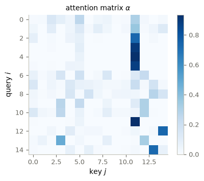
2. Why the \(1/\sqrt{d_a}\)
Suppose the entries of \(Q_i\) and \(K_j\) are independent with mean \(0\) and variance \(1\). Then \[ \langle Q_i, K_j \rangle = \sum_{\ell=1}^{d_a} Q_{i\ell} K_{j\ell} \quad\Longrightarrow\quad \mathbb{E}\big[\langle Q_i, K_j\rangle\big] = 0, \qquad \operatorname{Var}\big[\langle Q_i, K_j\rangle\big] = d_a . \] The logits therefore have typical size \(\sqrt{d_a}\), which grows with the model. A softmax fed logits of size \(\sqrt{d_a} \gg 1\) collapses onto a single entry, and its Jacobian \[ \frac{\partial \alpha_i}{\partial s_i} = \operatorname{diag}(\alpha_i) - \alpha_i \alpha_i^\top \] vanishes as \(\alpha_i \to\) one-hot: no gradient reaches \(W_Q\) and \(W_K\). Dividing by \(\sqrt{d_a}\) normalizes the variance back to \(1\), so the logits stay \(\mathcal{O}(1)\) at every width.
We can see the collapse directly by measuring the entropy \(H(\alpha_i) = -\sum_j \alpha_{ij}\log \alpha_{ij}\) of the attention rows, whose maximum \(\log n\) corresponds to uniform attention.
n, ds = 64, [2, 4, 8, 16, 32, 64, 128, 256, 512, 1024]
entropy = {True: [], False: []}
for d in ds:
    Q, K = torch.randn(n, d), torch.randn(n, d)
    for scaled in (True, False):
        A = (Q @ K.T / (d ** 0.5 if scaled else 1.0)).softmax(dim=1)
        entropy[scaled].append(-(A * A.clamp_min(1e-12).log()).sum(1).mean().item())

fig, ax = P.panels(figsize=(5.5, 3.4))
P.curves(ax, ds, {r"$QK^\top$": (entropy[False], {"color": P.ORANGE, "marker": "o"}),
                  r"$QK^\top/\sqrt{d_a}$": (entropy[True], {"color": P.BLUE, "marker": "o"})},
         log="x", xlabel="$d_a$", ylabel="mean row entropy (nats)")
ax.axhline(np.log(n), ls="--", color=P.INK, lw=1)
ax.text(2.2, np.log(n) - 0.4, "uniform attention, $\\log n$", fontsize=8)
plt.show()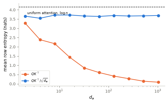
3. Multi-head attention
One attention map can only express one notion of relevance. Multi-head attention runs \(h\) independent copies in parallel, each in a subspace of width \(d_m/h\), and concatenates the results: \[ \operatorname{MHA}(X) = \big[\,H_1 \;\|\; \cdots \;\|\; H_h\,\big]\, W_O, \qquad H_m = \operatorname{Attn}\!\big(X W_Q^{(m)},\, X W_K^{(m)},\, X W_V^{(m)}\big), \] with \(W_O \in \mathbb{R}^{d_m \times d_m}\). Because \(d_a = d_v = d_m/h\), the leading-order projection and attention arithmetic is comparable to a single head of full width. Storing a separate attention map for each head still uses more memory. What they buy is rank: each \(W_Q^{(m)} W_K^{(m)\top}\) is a bilinear form of rank at most \(d_m/h\), so the model gets \(h\) different low-rank comparisons instead of one. Empirically the heads specialize.
In code, the three projections are fused into one Linear and the head axis is just a reshape.
def attention(Q, K, V):                                  # Q,K,V: [..., n, d]
    A = (Q @ K.transpose(-2, -1) / K.shape[-1] ** 0.5).softmax(dim=-1)
    return A @ V, A

class MultiHeadAttention(nn.Module):
    def __init__(self, d_model, n_heads):
        super().__init__()
        self.h = n_heads
        self.qkv = nn.Linear(d_model, 3 * d_model)       # W_Q, W_K, W_V for all heads at once
        self.out = nn.Linear(d_model, d_model)           # W_O

    def forward(self, X):                                # X: [B, n, d_model]
        B, n, d = X.shape
        Q, K, V = self.qkv(X).view(B, n, 3, self.h, d // self.h).permute(2, 0, 3, 1, 4)
        Y, A = attention(Q, K, V)                        # Y: [B, h, n, d/h],  A: [B, h, n, n]
        return self.out(Y.transpose(1, 2).reshape(B, n, d)), A
4. Positional encoding
Here is the catch. Let \(P\) be an \(n \times n\) permutation matrix. Then \(Q \mapsto PQ\), \(K \mapsto PK\), \(V \mapsto PV\), the scores become \(P S P^\top\), and since the softmax acts row-wise, \[ \operatorname{Attn}(PX) = P\,\alpha\, P^\top \cdot P V = P\, \alpha V = P \operatorname{Attn}(X). \] Self-attention is permutation-equivariant, and so is everything else in the block (LayerNorm and the MLP act on each token separately). Without positional information, the block treats its inputs as an unordered collection: permuting them simply permutes its outputs. It cannot represent word-order relationships through attention alone.
X, perm = torch.randn(1, 6, 8), torch.randperm(6)
mha = MultiHeadAttention(d_model=8, n_heads=2)
with torch.no_grad():
    err = (mha(X)[0][:, perm] - mha(X[:, perm])[0]).abs().max()
print(f"|Attn(PX) - P Attn(X)| = {err:.2e}")
|Attn(PX) - P Attn(X)| = 5.96e-08Order must therefore be injected into the inputs. The original paper adds a fixed sinusoidal positional encoding to the token embeddings, \(h_p^{(0)} = E_{t_p} + PE_p\), with \[ PE_{p,\,2k} = \sin\!\left(\omega_k\, p\right), \qquad PE_{p,\,2k+1} = \cos\!\left(\omega_k\, p\right), \qquad \omega_k = 10000^{-2k/d_m}. \]
Some remarks on why this particular choice:
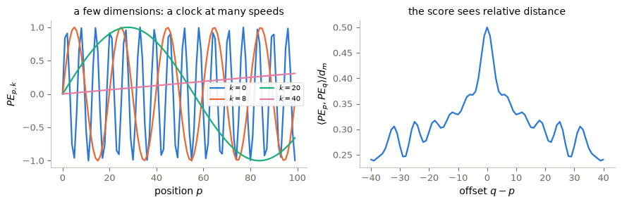
It is a clock at many speeds. Dimensions \((2k, 2k+1)\) trace the unit circle at angular frequency \(\omega_k\). The wavelengths \(2\pi/\omega_k\) form a geometric progression from \(2\pi\) to \(2\pi \cdot 10^4\), so the fast dimensions resolve immediate neighbors while the slow ones carry coarse global position — much like the bits of a binary counter, but smooth and bounded in \([-1,1]\).
Relative position is a linear map. From the angle-addition formulas, for every offset \(\Delta\) \[ \begin{pmatrix} \sin \omega_k (p+\Delta) \\ \cos \omega_k (p+\Delta) \end{pmatrix} = \underbrace{\begin{pmatrix} \cos \omega_k \Delta & \sin \omega_k \Delta \\ -\sin \omega_k \Delta & \cos \omega_k \Delta \end{pmatrix}}_{\text{rotation }R(\omega_k \Delta)} \begin{pmatrix} \sin \omega_k p \\ \cos \omega_k p \end{pmatrix} \qquad\Longrightarrow\qquad PE_{p+\Delta} = M_\Delta\, PE_p , \] where the block-diagonal \(M_\Delta\) does not depend on \(p\). So a linear layer inside \(W_Q\) can implement “attend \(\Delta\) positions back”, uniformly along the sequence. This is the property the encoding was designed for.
The score already knows about distance. Since \(\sin a \sin b + \cos a \cos b = \cos(a-b)\), \[ \langle PE_p, PE_q \rangle = \sum_k \cos\!\big(\omega_k (p-q)\big), \] a function of \(p-q\) alone, maximal at \(0\) but oscillatory, rather than monotonically decreasing with \(|p-q|\): a built-in “nearby tokens are relevant” prior, before any training.
It is fixed, not learned, so it is defined at positions never seen during training — the original motivation for extrapolating to longer sequences. In practice sinusoidal encodings extrapolate poorly, and modern models use learned embeddings or, most often, RoPE (Su et al., 2021), which applies the same rotation \(R(\omega_k \Delta)\) directly to \(Q\) and \(K\) so that the positional part of the interaction depends on the relative offset \(p-q\). The scores also depend on token content.
def positional_encoding(n, d):
    pos, i = torch.arange(n)[:, None], torch.arange(0, d, 2)[None, :]
    angle = pos / 10000 ** (i / d)                       # [n, d/2], omega_k * p
    PE = torch.zeros(n, d)
    PE[:, 0::2], PE[:, 1::2] = torch.sin(angle), torch.cos(angle)
    return PE

PE = positional_encoding(100, 64)

fig, ax = P.panels(figsize=(6, 3.0))
P.heatmap(ax, PE.T, cmap="RdBu_r", vmin=-1, vmax=1, aspect="auto",
          xlabel="position $p$", ylabel="dimension $k$",
          title="sinusoidal positional encoding $PE_{p,k}$")
plt.show()

fig, axes = P.panels(2, size=(4.5, 3.0))
P.curves(axes[0], None, {f"$k={k}$": (PE[:, k], c)
                         for k, c in zip([0, 8, 20, 40], [P.BLUE, P.ORANGE, P.AQUA, P.MAGENTA])},
         xlabel="position $p$", ylabel="$PE_{p,k}$",
         title="a few dimensions: a clock at many speeds", legend={"fontsize": 7, "ncol": 2})
offsets = np.arange(-40, 41)
P.curves(axes[1], offsets, [(PE[50] @ PE[50 + o]).item() / PE.shape[1] for o in offsets],
         xlabel="offset $q - p$", ylabel=r"$\langle PE_p, PE_q \rangle / d_m$",
         title="the score sees relative distance")
plt.show()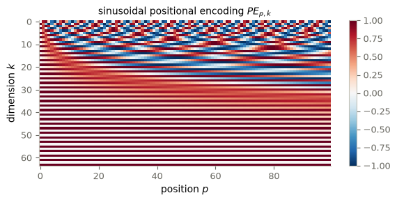
5. The transformer block
A block alternates mixing across tokens (attention) with mixing across features (a token-wise MLP), each wrapped in a residual connection around a LayerNorm: \[ \tilde h = h + \operatorname{MHA}\big(\operatorname{LN}(h)\big), \qquad h^{+} = \tilde h + \operatorname{MLP}\big(\operatorname{LN}(\tilde h)\big), \qquad \operatorname{MLP}(z) = W_2\, \sigma(W_1 z + b_1) + b_2 , \] with \(W_1 \in \mathbb{R}^{4 d_m \times d_m}\) (the usual expansion factor) and \(\sigma\) a GELU. Note:
- The residual stream \(h \mapsto h + f(h)\) is exactly the ResNet structure, i.e. one explicit Euler step of \(\dot h = f_\theta(h)\). A deep transformer is a discretized flow on a cloud of \(n\) interacting particles, where attention supplies the interaction between them. This is the starting point for the mean-field analyses of transformers (Geshkovski et al., 2023) and for §§7–11 below.
- Only attention moves information between positions; the MLP is applied independently at each token and holds most of the parameters (\(8 d_m^2\) against \(4 d_m^2\) for attention).
- Putting the LayerNorm inside the branch (“pre-LN”) keeps the residual path an exact identity and can improve gradient behavior and reduce the need for learning-rate warm-up (Xiong et al., 2020). The 2017 architecture used “post-LN” and a warm-up schedule.
class Block(nn.Module):
    def __init__(self, d_model, n_heads):
        super().__init__()
        self.ln1, self.ln2 = nn.LayerNorm(d_model), nn.LayerNorm(d_model)
        self.attn = MultiHeadAttention(d_model, n_heads)
        self.mlp = nn.Sequential(nn.Linear(d_model, 4 * d_model), nn.GELU(),
                                 nn.Linear(4 * d_model, d_model))

    def forward(self, X):
        Y, A = self.attn(self.ln1(X))
        X = X + Y                                        # attention  : mixes tokens
        return X + self.mlp(self.ln2(X)), A              # MLP        : mixes features

class TinyBERT(nn.Module):
    def __init__(self, vocab, n, d_model=64, n_heads=4, n_layers=2):
        super().__init__()
        self.emb = nn.Embedding(vocab, d_model)
        self.register_buffer("pe", positional_encoding(n, d_model))
        self.blocks = nn.ModuleList([Block(d_model, n_heads) for _ in range(n_layers)])
        self.ln, self.head = nn.LayerNorm(d_model), nn.Linear(d_model, vocab)

    def forward(self, tokens):                           # tokens: [B, n] of token ids
        X, maps = self.emb(tokens) + self.pe[:tokens.shape[1]], []
        for block in self.blocks:
            X, A = block(X)
            maps.append(A)
        return self.head(self.ln(X)), maps               # logits: [B, n, vocab]
6. BERT-style masked language modeling
BERT (Devlin et al., 2019) trains the encoder above as a denoiser. Corrupt a piece of text \(t = (t_1,\dots,t_n)\) by replacing the tokens at a random subset \(M \subset \{1,\dots,n\}\) with a special [MASK] symbol, call the result \(\tilde t\), and minimize \[
\mathcal{L}(\theta) = -\,\mathbb{E}_{t,\,M} \sum_{p \in M} \log p_\theta\big(t_p \mid \tilde t\big),
\qquad
p_\theta(\,\cdot \mid \tilde t) = \operatorname{softmax}\big(W\, h_p^{(L)} + b\big).
\] Because there is no causal mask, \(h_p^{(L)}\) sees the whole window — both sides of the gap. That is the difference from a GPT-style decoder, which masks the upper triangle of \(\alpha\) and predicts \(t_{p+1}\) from \(t_{\le p}\). BERT masks \(15\%\) of tokens; of those, \(80\%\) become [MASK], \(10\%\) a random word and \(10\%\) are left alone, so the model cannot simply ignore unmasked positions. We keep plain [MASK].
Tiny Shakespeare
The corpus is Tiny Shakespeare (Karpathy, 2015): about \(1.1\)M characters of Shakespeare’s plays in a single 1 MB text file. We tokenize by characters, so the vocabulary is the \(65\) characters that occur plus [MASK], and a training example is a random window of \(n = 64\) consecutive characters. The first \(10^6\) characters are for training; the last \(\approx 10^5\) are held out.
# Tiny Shakespeare: 1.1M characters of the plays, downloaded once into ./data
DATA = pathlib.Path("data"); DATA.mkdir(exist_ok=True)
path = DATA / "tinyshakespeare.txt"
if not path.exists():
    urllib.request.urlretrieve(
        "https://raw.githubusercontent.com/karpathy/char-rnn/master/data/tinyshakespeare/input.txt", path)
text = path.read_text()

VOCAB = ["[MASK]"] + sorted(set(text))                      # one token per character
stoi, MASK, N = {c: i for i, c in enumerate(VOCAB)}, 0, 64
data = torch.tensor([stoi[c] for c in text])
train, test = data[:1_000_000], data[1_000_000:]
show = lambda ids: "".join("_" if i == MASK else VOCAB[i] for i in ids)

def windows(src, B):                                         # B random windows of N characters
    i = torch.randint(0, len(src) - N, (B, 1))
    return src[i + torch.arange(N)]

print(f"{len(text):,} characters, vocabulary {len(VOCAB)}, window n = {N}")
for w in windows(train, 3):
    print("-" * 64 + "\n" + show(w))
1,115,394 characters, vocabulary 66, window n = 64
----------------------------------------------------------------
must what force will have us do.
Set on towards London, cousin,
----------------------------------------------------------------
know each other's faces,
But for our hearts, he knows no more of
----------------------------------------------------------------
ert thou regent of the world,
It were a shame to let this land bMasking is three lines: draw a Bernoulli\((0.15)\) mask, hide those tokens, and set every unmasked target to -100 so that cross_entropy ignores it — the loss lives only on the holes. We add one line that is not in BERT: the last character of every window is always hidden as well. A hole in the middle of a window sees text on both sides, but generation (below) asks the opposite question — the next character, with nothing to its right — and without this line the model would meet it only in the few windows whose last character happens to be drawn.
def corrupt(x):
    tokens, target = x.clone(), x.clone()
    m = torch.rand(x.shape) < 0.15
    m[:, -1] = True                                          # always hide the last character too
    tokens[m], target[~m] = MASK, -100                       # hide the token, score only the holes
    return tokens, target

model = TinyBERT(len(VOCAB), N)
opt = torch.optim.Adam(model.parameters(), lr=3e-3)
print("parameters:", sum(p.numel() for p in model.parameters()))

losses, accs = [], []
for it in range(2001):
    tokens, target = corrupt(windows(train, 64))
    logits, _ = model(tokens)
    L = nn.functional.cross_entropy(logits.reshape(-1, len(VOCAB)), target.reshape(-1))
    opt.zero_grad(); L.backward(); opt.step()
    losses.append(L.item())
    if it % 100 == 0:                                        # held-out text, never trained on
        with torch.no_grad():
            tk, tg = corrupt(windows(test, 512))
            hole = tg != -100
            accs.append((model(tk)[0].argmax(-1)[hole] == tg[hole]).float().mean().item())
        if it % 500 == 0:
            print(f"iteration {it:4d}:  loss = {L.item():.3f},  test accuracy on masked characters = {accs[-1]:.1%}")

fig, axes = P.panels(2, size=(4.5, 3.0))
P.curves(axes[0], None, P.smooth(losses, 25), xlabel="iteration", ylabel="MLM loss",
         title="training loss")
P.curves(axes[1], np.arange(len(accs)) * 100, (accs, {"color": P.ORANGE, "marker": "o", "ms": 3}),
         xlabel="iteration", ylabel="accuracy", ylim=(0, 1),
         title="held-out accuracy on masked characters")
plt.show()
parameters: 108610
iteration 0: loss = 4.380, test accuracy on masked characters = 14.9%
iteration 500: loss = 2.506, test accuracy on masked characters = 30.5%
iteration 1000: loss = 1.756, test accuracy on masked characters = 45.5%
iteration 1500: loss = 1.540, test accuracy on masked characters = 49.4%
iteration 2000: loss = 1.523, test accuracy on masked characters = 51.2%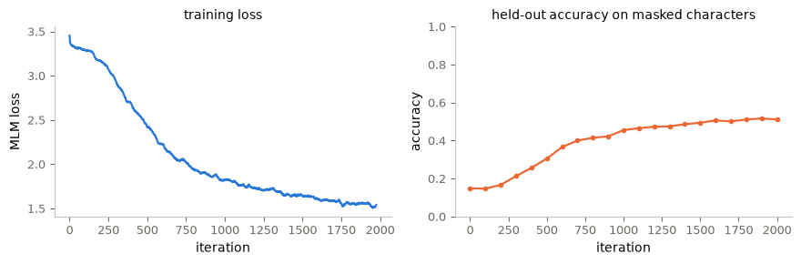
Filling in the blanks
Hide a single character of held-out text, the e in see the like, and ask the model for it. The shaded slot holds its most likely character; the bars show the whole distribution, the hidden character in orange.
i = text.index("Peter, didst ever see the like?", 1_000_000)  # a line of held-out text
x, hole = data[i : i + N], len("Peter, didst ever see th")     # a window, and the e of "the"
tokens = x.clone(); tokens[hole] = MASK
with torch.no_grad():
    logits, _ = model(tokens[None])
P.fill_in(show(x), hole, logits[0, hole].softmax(-1), VOCAB)
plt.show()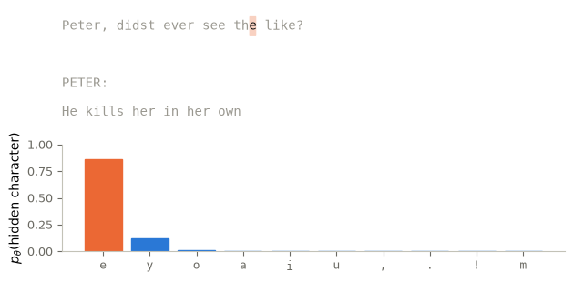
Writing, one character at a time
Any distribution over strings factorizes by the chain rule, \[
p(t_1, \dots, t_T) = \prod_{k=1}^{T} p\big(t_k \mid t_1, \dots, t_{k-1}\big),
\] so a model of the next character is a generative model: sample \(t_k\), append it, and repeat. Our BERT supplies that conditional — feed it the last \(n-1\) characters followed by a [MASK] and read the distribution at the hole, \[
p_\theta\big(t_k \mid t_{k-n+1}, \dots, t_{k-1}\big)
= \operatorname{softmax}\big(W h_n^{(L)} + b\big)
\quad\text{on the input}\quad \big(t_{k-n+1}, \dots, t_{k-1}, \texttt{[MASK]}\big).
\] The window slides along, so the model never sees more than the last \(63\) characters. We sample at temperature \(\tau = 0.8\), i.e. from \(\operatorname{softmax}(\text{logits}/\tau)\), which sharpens the distribution slightly.
This is exactly the task a GPT-style decoder is trained on — at every position of every window at once, thanks to the causal mask — whereas our BERT practises it once per window. That is why generation belongs to decoders, and why a two-minute BERT writes Shakespeare only in texture.
def generate(prompt, steps, tau=0.8):
    ids, probs = [stoi[c] for c in prompt], []
    for _ in range(steps):
        x = torch.tensor(ids[-(N - 1):] + [MASK])               # the last n-1 characters, then a hole
        with torch.no_grad():
            p = (model(x[None])[0][0, -1] / tau).softmax(-1)
        ids.append(torch.multinomial(p, 1).item()); probs.append(p)
    return ids[len(prompt):], torch.stack(probs)

torch.manual_seed(0)

prompt = "JULIET:\nO Romeo, Romeo! wherefore art thou"
sampled, probs = generate(prompt, 60)
P.animate_generation(prompt, sampled, probs, VOCAB)7. Tokens as interacting particles: hardmax attention
We now strip the transformer to its interaction. Keep only attention (no feed-forward block, no LayerNorm, no heads), fix the matrices, and replace the softmax by its zero-temperature limit. A sentence is a collection \(Z=\{z_1,\dots,z_n\}\subset\mathbb R^d\) of tokens, and each layer is
- self-attention: \(\displaystyle y_i=z_i+\sum_{j=1}^n\Lambda^A_{ij}(Z)\,Vz_j\), with weights \(\Lambda^A_{ij}(Z)\ge0\), \(\sum_j\Lambda^A_{ij}(Z)=1\), favouring the tokens \(z_j\) that score highest against \(z_i\) in the bilinear form \(\langle Az_i,z_j\rangle\).
Hardmax self-attention. Each token attends, with equal weights, to the tokens that score highest against it: \[ y_i=z_i+\frac{1}{|\mathcal C_i(Z)|}\sum_{j\in\mathcal C_i(Z)}Vz_j,\qquad \mathcal C_i(Z)=\Big\{j\in[n]:\ \langle Az_i,z_j\rangle=\max_{\ell\in[n]}\langle Az_i,z_\ell\rangle\Big\}. \] The set \(\mathcal C_i(Z)\) contains all maximizers. When several tokens tie, token \(i\) averages over all of them. In floating point, \(j\) counts as a maximizer when \(\langle Az_i,z_j\rangle\ge\max_\ell\langle Az_i,z_\ell\rangle-\mathrm{rtol}\cdot\max\big(1,|\max_\ell\langle Az_i,z_\ell\rangle|\big)\) with \(\mathrm{rtol}=10^{-12}\), so that exact ties remain ties. This tie tolerance is unrelated to the distance tolerance \(10^{-6}\) used in §10 to count clusters. A token is a leader if \(\mathcal C_i(Z)=\{i\}\): it scores strictly highest against itself.
Assumptions on the matrices: (i) \(A\) is symmetric and positive definite; (ii) \(V=\alpha I\) with a step size \(\alpha>0\).
The normalized update. With \(V=\alpha I\) and \(m_i=\frac1{|\mathcal C_i|}\sum_{j\in\mathcal C_i}z_j\), the layer gives \(y_i=z_i+\alpha m_i\). A leader has \(m_i=z_i\), so \(y_i=(1+\alpha)z_i\): without further action, leaders would be multiplied by \(1+\alpha\) at every layer. Dividing by \(1+\alpha\) removes this growth and gives the pure-attention hardmax transformer: \[ \boxed{\;z_i^{k+1}=\frac{z_i^k+\alpha\,m_i^k}{1+\alpha}=z_i^k+\frac{\alpha}{1+\alpha}\Big(\frac1{|\mathcal C_i(Z^k)|}\sum_{j\in\mathcal C_i(Z^k)}z_j^k-z_i^k\Big).\;} \] Each new token is a convex combination of current tokens: weight \(\frac1{1+\alpha}\) on itself and \(\frac{\alpha}{1+\alpha}\) shared equally by its maximizers. The second form shows a residual step of size \(\frac{\alpha}{1+\alpha}\) towards the average of the attended tokens.
Predict. Three tokens \(z_1=(2,0)\), \(z_2=(0,1)\), \(z_3=(1,0.5)\), with \(A=I\), \(\alpha=0.1\). Which are leaders, and where does \(z_3\) go in one step? And for \(z_1=(1,0)\), \(z_2=(0,1)\), \(z_3=(\frac12,\frac12)\)?
def scores(Z, A):
    return (Z @ A) @ Z.T                                 # scores[i, j] = <A z_i, z_j>

def hardmax_sets(Z, A, rtol=1e-12):
    S = scores(Z, A)
    cut = S.max(axis=1) - rtol * np.maximum(1.0, np.abs(S.max(axis=1)))
    return [np.where(S[i] >= cut[i])[0] for i in range(len(Z))]

def leaders(Z, A, rtol=1e-12):
    return np.array([i for i, Ci in enumerate(hardmax_sets(Z, A, rtol)) if len(Ci) == 1 and Ci[0] == i])

def hardmax_step(Z, A, alpha):
    m = np.array([Z[Ci].mean(axis=0) for Ci in hardmax_sets(Z, A)])
    return (Z + alpha * m) / (1 + alpha)

def hardmax_flow(Z0, A, alpha, K):
    traj = [Z0]
    for _ in range(K):
        traj.append(hardmax_step(traj[-1], A, alpha))
    return np.array(traj)

def attention_layer(Z, A, V):                            # the unnormalized layer: y_i = z_i + mean_{C_i} V z_j
    return Z + np.array([(Z[Ci] @ V.T).mean(axis=0) for Ci in hardmax_sets(Z, A)])

A_toy, alpha_toy, K_toy = np.eye(2), 0.1, 40             # parameters of the toy-token experiments

for name, Z in (("z1=(2,0), z2=(0,1), z3=(1,0.5)", np.array([[2.0, 0.0], [0.0, 1.0], [1.0, 0.5]])),
                ("z1=(1,0), z2=(0,1), z3=(1/2,1/2)", np.array([[1.0, 0.0], [0.0, 1.0], [0.5, 0.5]]))):
    print(f"{name}:  scores <A z_i, z_j> =\n{scores(Z, A_toy)}")
    print("  attended sets C_i:", [[int(j) + 1 for j in Ci] for Ci in hardmax_sets(Z, A_toy)],
          "  leaders:", [int(i) + 1 for i in leaders(Z, A_toy)])
    print("  one step:", hardmax_step(Z, A_toy, alpha_toy).round(4).tolist())
    print("  normalized unrestricted layer gives the same:",
          bool(np.allclose(attention_layer(Z, A_toy, alpha_toy * np.eye(2)) / (1 + alpha_toy),
                           hardmax_step(Z, A_toy, alpha_toy))))
z1=(2,0), z2=(0,1), z3=(1,0.5): scores <A z_i, z_j> =
[[4. 0. 2. ]
[0. 1. 0.5 ]
[2. 0.5 1.25]]
attended sets C_i: [[1], [2], [1]] leaders: [1, 2]
one step: [[2.0, 0.0], [0.0, 1.0], [1.0909, 0.4545]]
normalized unrestricted layer gives the same: True
z1=(1,0), z2=(0,1), z3=(1/2,1/2): scores <A z_i, z_j> =
[[1. 0. 0.5]
[0. 1. 0.5]
[0.5 0.5 0.5]]
attended sets C_i: [[1], [2], [1, 2, 3]] leaders: [1, 2]
one step: [[1.0, 0.0], [0.0, 1.0], [0.5, 0.5]]
normalized unrestricted layer gives the same: TrueReading the output (answer to the prediction). - First configuration. Token 3 scores \(2\) against \(z_1\), \(0.5\) against \(z_2\) and \(1.25\) against itself, so \(\mathcal C_3=\{1\}\), and it moves to \(\big((1,0.5)+0.1\,(2,0)\big)/1.1\approx(1.091,0.455)\). Tokens 1 and 2 are leaders and do not move. - Second configuration. Token 3 scores exactly \(\frac12\) against all three tokens: \(\mathcal C_3=\{1,2,3\}\), the average is \((\frac12,\frac12)\) itself, and token 3 does not move either. It is not a leader, yet it is at rest. It sits at the point of the segment \([z_1,z_2]\) closest to the origin, a configuration that will reappear in the theorem of §9. - Ties. A rule that picked only one maximizer, say the first, would move token 3 towards \(z_1\) and give a different dynamics. Keeping all maximizers is part of the model.
8. Two facts, with proofs
Both proofs use only the convex-combination form of the update.
Fact 1 (the convex hull shrinks). For any matrix \(A\) and \(\alpha>0\), every token of \(Z^{k+1}\) lies in the convex hull of \(Z^k\). Hence all tokens stay forever in the convex hull of the initial tokens, and these hulls are nested.
Proof. \(z_i^{k+1}=\frac1{1+\alpha}z_i^k+\frac{\alpha}{1+\alpha}\cdot\frac1{|\mathcal C_i|}\sum_{j\in\mathcal C_i}z_j^k\) has non-negative weights summing to \(1\). \(\square\)
Fact 2 (leaders stay leaders and do not move). If \(i\) is a leader of \(Z^k\), then \(z_i^{k+1}=z_i^k\) and \(i\) is a leader of \(Z^{k+1}\). By induction, a leader of \(Z^0\) never moves.
Proof. Since \(\mathcal C_i=\{i\}\), \(m_i=z_i^k\), so \(z_i^{k+1}=(z_i^k+\alpha z_i^k)/(1+\alpha)=z_i^k\). Write \(z_i=z_i^k\) and \(c_\ell=\langle Az_i,z_\ell^k\rangle\); being a leader means \(c_i>c_\ell\) for all \(\ell\ne i\). For \(j\ne i\), \(z_j^{k+1}=\sum_\ell\lambda_\ell z_\ell^k\) is a convex combination in which \(z_j^k\) itself has weight at least \(\frac1{1+\alpha}>0\), so the weight \(\lambda_i\) on \(z_i\) is at most \(\frac{\alpha}{1+\alpha}<1\). Then \[ \langle Az_i^{k+1},z_j^{k+1}\rangle=\sum_\ell\lambda_\ell c_\ell<c_i=\langle Az_i^{k+1},z_i^{k+1}\rangle, \] strictly, because some weight sits on indices \(\ell\ne i\), where \(c_\ell<c_i\). So \(i\) is still the unique maximizer of its own row. \(\square\)
A consequence: the geometric rate of followers. If, from some layer on, a token \(j\) attends only to a leader \(i\) (\(\mathcal C_j=\{i\}\)), then \(z_j^{k+1}-z_i=\frac{1}{1+\alpha}(z_j^k-z_i)\). Its distance to the leader shrinks by the factor \(\frac1{1+\alpha}\) per layer, never reaching zero in exact arithmetic. With \(\alpha=0.1\), forty layers shrink it only to \(1.1^{-40}\approx0.022\) of its initial value.
What the proofs do not use. Neither needs \(A\) to be symmetric or positive definite, nor the tokens to be distinct or nonzero. Those hypotheses enter the theorem below, which says much more: that every token converges.
9. The clustering theorem and what it assumes
Theorem (Alcalde, Fantuzzi and Zuazua, 2025), transcribed. Let \(z_1^0,\dots,z_n^0\in\mathbb R^d\) be nonzero and distinct, and \(A\in\mathbb R^{d\times d}\) symmetric positive definite. There exists a finite set \(\mathcal S=\{s_1,\dots,s_p\}\subset\mathbb R^d\), \(p\le n\), such that for every \(i\in[n]\), \(z_i^K\to s\in\mathcal S\) as \(K\to\infty\). Moreover, the first \(m\le p\) elements of \(\mathcal S\) are the vertices of a convex polytope \(\mathcal K\), which are the leaders, and the remaining elements are the projections of the origin (with respect to \(\|\cdot\|_A\)) onto the faces of \(\mathcal K\).
Audit. - Hypotheses. The hypotheses are on the initial tokens and on \(A\); \(\alpha>0\) is arbitrary. Nonzero matters because the token \(0\) scores \(\langle A0,z_j\rangle=0\) against every token: all tokens tie for it, and it moves to the average of the configuration (Exercise 7). Distinct matters because identical tokens always tie with each other. - The conclusion is asymptotic. It gives no rate and no number of layers after which the tokens are close to \(\mathcal S\); with \(K=40\), nothing is guaranteed. - “Which are the leaders”. The statement does not say when these tokens are leaders. Fact 2 proves only persistence: a token that is a leader at layer \(k\) stays fixed and remains a leader from layer \(k\) on. It does not prove that every leader of the limit configuration was already a leader at \(k=0\). Leadership can emerge, as the example below shows. Our reading: the leaders of the conclusion are the tokens that are leaders from some layer on. - The other limit points are projections of the origin onto faces of \(\mathcal K\). The second configuration of §7 is an example: token 3 rests at the projection of \(0\) onto the edge \([z_1,z_2]\). - What is not stated. The theorem says neither which token goes to which limit, nor how the limits depend on \(\alpha\). It concerns pure hardmax attention, not the transformer with feed-forward blocks or softmax weights.
Leadership can emerge. Take \(A=I\), \(\alpha=0.1\) and the four tokens of the cell below. Initially, token 2 scores \(0.3877\) against itself and \(0.3905\) against token 4, so it is not a leader; the leaders are tokens 1 and 3. After one layer, token 2 has moved to \((0.3409\ldots,0.5227\ldots)\). Its own score, \(\approx0.38946\), now exceeds its score against the moved token 4, \(\approx0.38277\): it has become a leader. By Fact 2 it stays fixed from then on, in exact arithmetic. This is not a rounding effect; the cell checks it with the scores computed by an independent matrix product, with tolerance \(0\) and with the tolerance \(10^{-12}\).
Z_em = np.array([[0.18, -0.95], [0.31, 0.54], [1.45, -0.63], [0.65, 0.35]])
Z_em1 = hardmax_step(Z_em, A_toy, alpha_toy)
for name, Zk in (("initial", Z_em), ("after one layer", Z_em1)):
    S_k = Zk @ Zk.T                                      # scores by an independent matrix product (A = I)
    print(f"{name:16s} row of token 2: {S_k[1].round(8)};  leaders (1-based) with rtol = 0: "
          f"{[int(i) + 1 for i in leaders(Zk, A_toy, rtol=0.0)]}, "
          f"with rtol = 1e-12: {[int(i) + 1 for i in leaders(Zk, A_toy)]}")
print("token 2 after one layer:", Z_em1[1].round(4), "  after two layers:",
      hardmax_step(Z_em1, A_toy, alpha_toy)[1].round(4))
initial row of token 2: [-0.4572 0.3877 0.1093 0.3905]; leaders (1-based) with rtol = 0: [1, 3], with rtol = 1e-12: [1, 3]
after one layer row of token 2: [-0.43522727 0.38946281 0.165 0.3827686 ]; leaders (1-based) with rtol = 0: [1, 2, 3], with rtol = 1e-12: [1, 2, 3]
token 2 after one layer: [0.3409 0.5227] after two layers: [0.3409 0.5227]10. Laboratory: toy tokens, forty layers and beyond
Set-up (fixed before the experiment). - Tokens. The toy tokens: two collections of 13 tokens, drawn uniformly in \([-1,1]^2\) from this notebook’s generator. The cell checks that the tokens are nonzero and distinct. - Parameters. \(A=I\), \(\alpha=0.1\), \(K=40\); then \(K=400\) and \(4000\). - Tolerances, fixed in advance. Maximizer sets use the relative tolerance \(10^{-12}\); two tokens count as one cluster when they are within \(10^{-6}\).
Predict. After 40 layers, will the tokens have reached a finite set of points? How many clusters do you expect, and where?
from scipy.spatial import ConvexHull

def convex_hull_2d(pts):
    return ConvexHull(pts).vertices                      # indices in counter-clockwise order

def in_convex_hull(pts, hull_pts, tol=1e-9):
    v = hull_pts[convex_hull_2d(hull_pts)]
    edges = np.roll(v, -1, axis=0) - v                   # CCW edges: inside means cross >= 0 for every edge
    rel = pts[:, None, :] - v[None, :, :]
    cross = edges[None, :, 0] * rel[:, :, 1] - edges[None, :, 1] * rel[:, :, 0]
    return np.all(cross >= -tol, axis=1)

collections = [rng.uniform(-1, 1, (13, 2)) for _ in range(2)]
K_long = 4000

def clusters(Z, tol=1e-6):
    reps = []
    for z in Z:
        if not any(np.linalg.norm(z - r) < tol for r in reps):
            reps.append(z)
    return np.array(reps)

runs = []
for c, Z0 in enumerate(collections):
    dist = min(np.linalg.norm(Z0[i] - Z0[j]) for i in range(len(Z0)) for j in range(i))
    traj = hardmax_flow(Z0, A_toy, alpha_toy, K_long)
    L0 = leaders(Z0, A_toy)
    final = traj[-1]
    # Colouring rule for THESE draws: nearest initial leader after 4000 layers. Whether every limit IS an
    # initial leader is exactly what the printed distances check; an emergent leader or a face projection
    # would show up as a large distance.
    follow = np.array([L0[np.argmin(np.linalg.norm(Z0[L0] - z, axis=1))] for z in final])
    runs.append({"Z0": Z0, "traj": traj, "leaders": L0, "follow": follow})
    print(f"collection {c + 1}: smallest |z_i| = {np.linalg.norm(Z0, axis=1).min():.3f}, "
          f"smallest distance = {dist:.3f} (nonzero, distinct); "
          f"initial leaders (1-based): {[int(i) + 1 for i in L0]}")
    for K in (K_toy, 400, K_long):
        res = np.abs(traj[K] - traj[K - 1]).max()
        reps = clusters(traj[K])
        gap = np.abs(traj[K][:, None, :] - Z0[L0][None, :, :]).max(axis=2).min(axis=1).max()
        print(f"   K = {K:5d}: residual max|z^K - z^(K-1)| = {res:.1e},  clusters {len(reps):2d},  "
              f"largest distance of a token to the nearest initial leader {gap:.1e}")
    moved = np.abs(traj[:, L0] - Z0[L0]).max(axis=(1, 2))   # leaders' displacement (exact arithmetic: 0)
    print(f"   largest displacement of the initial leaders: {moved[K_toy]:.1e} after {K_toy} layers, "
          f"{moved[-1]:.1e} after {K_long};  all tokens inside the initial convex hull at every layer: "
          f"{bool(all(np.all(in_convex_hull(Z, Z0)) for Z in traj))}")

palette = [P.BLUE, P.ORANGE, P.MAGENTA, P.AQUA, "#8064a2", "#f79646", "#4bacc6"]
fig, axes = P.panels(2, figsize=(11, 4.6))
for ax, run in zip(axes, runs):
    traj, L0 = run["traj"][:K_toy + 1], run["leaders"]
    colour = {int(l): palette[k % len(palette)] for k, l in enumerate(L0)}
    for i in range(traj.shape[1]):
        ax.plot(traj[:, i, 0], traj[:, i, 1], "-", color=colour[int(run["follow"][i])], lw=1)
        ax.plot(*traj[0, i], "o", mfc="white", color=colour[int(run["follow"][i])], ms=5)
        ax.plot(*traj[-1, i], "o", color=colour[int(run["follow"][i])], ms=4)
    ax.plot(run["Z0"][L0, 0], run["Z0"][L0, 1], "*", color=P.INK, ms=13, mfc="gold")
    hull = L0[convex_hull_2d(run["Z0"][L0])]
    ax.plot(*np.vstack([run["Z0"][hull], run["Z0"][hull[:1]]]).T, ":", color=P.GREY, lw=1)
    ax.plot(0, 0, "+", color=P.INK)
    P.label(ax, equal=True, title=f"K = {K_toy} layers")
plt.show()
collection 1: smallest |z_i| = 0.536, smallest distance = 0.027 (nonzero, distinct); initial leaders (1-based): [2, 4, 5, 6, 8]
K = 40: residual max|z^K - z^(K-1)| = 1.4e-03, clusters 13, largest distance of a token to the nearest initial leader 1.4e-02
K = 400: residual max|z^K - z^(K-1)| = 0.0e+00, clusters 5, largest distance of a token to the nearest initial leader 1.6e-12
K = 4000: residual max|z^K - z^(K-1)| = 0.0e+00, clusters 5, largest distance of a token to the nearest initial leader 1.6e-12
largest displacement of the initial leaders: 4.4e-16 after 40 layers, 1.6e-12 after 4000; all tokens inside the initial convex hull at every layer: True
collection 2: smallest |z_i| = 0.177, smallest distance = 0.204 (nonzero, distinct); initial leaders (1-based): [4, 7, 9, 11, 12, 13]
K = 40: residual max|z^K - z^(K-1)| = 1.7e-03, clusters 13, largest distance of a token to the nearest initial leader 1.7e-02
K = 400: residual max|z^K - z^(K-1)| = 0.0e+00, clusters 6, largest distance of a token to the nearest initial leader 1.1e-12
K = 4000: residual max|z^K - z^(K-1)| = 0.0e+00, clusters 6, largest distance of a token to the nearest initial leader 1.1e-12
largest displacement of the initial leaders: 6.7e-16 after 40 layers, 1.1e-12 after 4000; all tokens inside the initial convex hull at every layer: True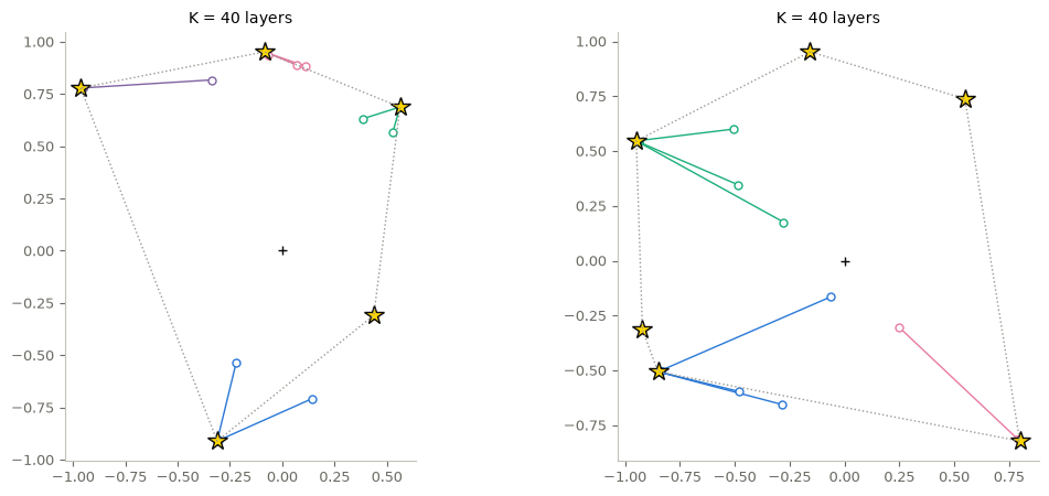
Figure (toy tokens). Two collections of 13 tokens (open circles) after \(K=40\) layers of the pure-attention hardmax transformer, \(A=I\), \(\alpha=0.1\) (filled circles: positions at layer 40). Stars are the leaders of the initial configuration, the dotted polygon their convex hull, and \(+\) the origin. Each token is coloured by the initial leader it is closest to after 4000 layers.
Interpretation (answer to the prediction). Leaders do not move (Fact 2): their printed displacement after 40 layers is at the level of rounding, since \((z+0.1z)/1.1\) is not exactly \(z\) in floating point. Every other token moves inside the convex hull (Fact 1, checked) towards its limit. The printed distances to the nearest initial leader say whether every limit observed here is an initial leader, or whether an emergent leader or a face projection appears; the colouring by nearest initial leader is valid for these draws only. After 40 layers the clusters are forming but not reached: the printed residual is far above rounding, and more than the final number of distinct positions remain at the tolerance \(10^{-6}\).
fig, (ax1, ax2) = P.panels(2, figsize=(11, 3.8))
for c, (run, col) in enumerate(zip(runs, (P.BLUE, P.ORANGE))):
    traj = run["traj"][:601]
    res = np.abs(np.diff(traj, axis=0)).max(axis=(1, 2))
    n_clusters = [len(clusters(Z)) for Z in traj]
    n_leaders = [len(leaders(Z, A_toy)) for Z in traj]
    ax1.semilogy(np.arange(1, len(res) + 1), np.maximum(res, 1e-18), color=col, label=f"collection {c + 1}")
    ax2.plot(n_clusters, color=col, label=f"collection {c + 1}: clusters (tol. $10^{{-6}}$)")
    ax2.plot(n_leaders, "--", color=col, lw=1, label=f"collection {c + 1}: tokens with $\\mathcal{{C}}_i=\\{{i\\}}$")
    print(f"collection {c + 1}: clusters at K = 40, 100, 200, 400, 600: "
          f"{[n_clusters[k] for k in (40, 100, 200, 400, 600)]}")
k = np.arange(1, 601)
ax1.semilogy(k, 0.5 * 1.1 ** (-k.astype(float)), ":", color=P.GREY, label=r"$(1+\alpha)^{-k}$")
ax1.axvline(K_toy, color=P.RULE, lw=0.7)
P.label(ax1, "layer $k$", r"$\max_i|z_i^{k}-z_i^{k-1}|$", ylim=(1e-18, 1))
ax2.axvline(K_toy, color=P.RULE, lw=0.7)
P.label(ax2, "layer $k$", "count")
plt.show()
collection 1: clusters at K = 40, 100, 200, 400, 600: [13, 13, 5, 5, 5]
collection 2: clusters at K = 40, 100, 200, 400, 600: [13, 13, 6, 6, 6]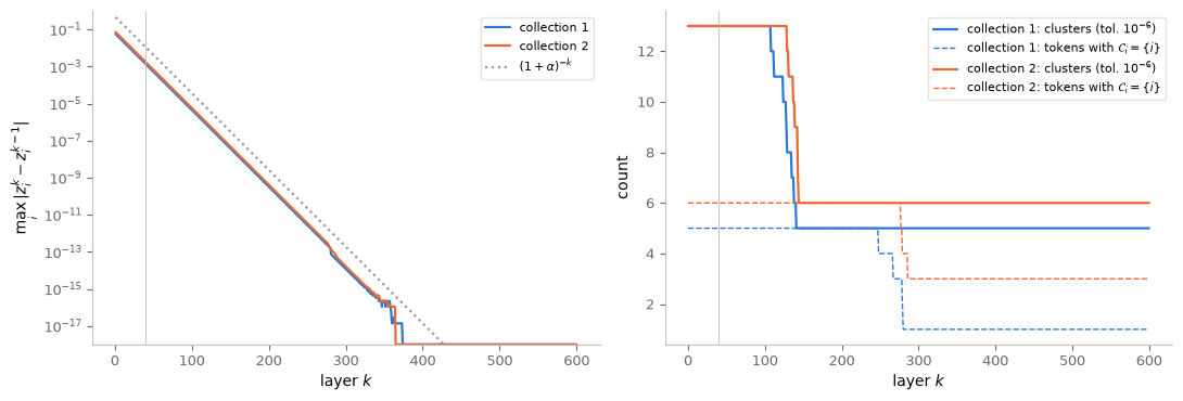
Figure (toy tokens, long run). Left: the residual \(\max_i|z_i^k-z_i^{k-1}|\) against the layer, with the rate \((1+\alpha)^{-k}\) of a follower attending to a fixed leader; the vertical line marks \(K=40\). Right: the number of clusters (distance tolerance \(10^{-6}\)) and, dashed, the number of tokens that are strict leaders, \(\mathcal C_i=\{i\}\).
Interpretation. After the last change of attended sets, the residual decays at the geometric rate \((1+\alpha)^{-k}\) computed in §8; the plot floors it at \(10^{-18}\). The number of clusters drops to its final value after a few hundred layers (printed), far beyond \(K=40\). The dashed curves and the printed leader displacements show artefacts of finite precision and of the tie tolerance fixed in advance, not of the mathematics: when a follower comes within the relative tolerance \(10^{-12}\) of its leader, the two are treated as tied; the leader then no longer satisfies \(\mathcal C_i=\{i\}\), and it moves by amounts of order \(10^{-12}\) towards its follower. Soon after, rounding leaves every token unchanged: the residual becomes exactly \(0\) with followers still about \(10^{-12}\) from their leaders. In exact arithmetic followers never reach their leaders and leaders never move (§8). These are observations of finitely many layers in floating point; they illustrate the theorem, they do not prove it.
11. Softmax at low temperature, and ties
Practical transformers use softmax weights \(\Lambda_{ij}=e^{\beta\langle Az_i,z_j\rangle}/\sum_\ell e^{\beta\langle Az_i,z_\ell\rangle}\), with an inverse temperature \(\beta\). As \(\beta\to\infty\), the weights concentrate on the maximizers. If the largest score is attained at \(q\) tokens and the next score is lower by a gap \(g>0\), each maximizer receives weight \(\frac1q+O(e^{-\beta g})\) and every other token \(O(e^{-\beta g})\). In the limit, the weights are uniform on all maximizers, which is exactly the hardmax rule with ties of §7. A rule that chose one maximizer would not be the limit of softmax. The cell compares one softmax step with one hardmax step, for the tie configuration of §7 and for the first collection of toy tokens, as \(\beta\) grows.
def softmax_step(Z, A, alpha, beta):
    S = beta * scores(Z, A)
    W = np.exp(S - S.max(axis=1, keepdims=True))
    W = W / W.sum(axis=1, keepdims=True)
    return (Z + alpha * W @ Z) / (1 + alpha)

Z_tie = np.array([[1.0, 0.0], [0.0, 1.0], [0.5, 0.5], [-0.4, 0.2]])
betas = np.array([1, 3, 10, 30, 100, 300, 1000])
fig, ax = P.panels(figsize=(6.6, 3.6))
for name, Z, col in (("tie configuration of section 7 (+ one token)", Z_tie, P.BLUE),
                     ("toy tokens, collection 1", runs[0]["Z0"], P.ORANGE)):
    dev = [np.abs(softmax_step(Z, A_toy, alpha_toy, b) - hardmax_step(Z, A_toy, alpha_toy)).max() for b in betas]
    S = scores(Z, A_toy)
    srt = np.sort(S, axis=1)[:, ::-1]
    gaps = [row[0] - row[row < row[0] - 1e-12 * max(1, abs(row[0]))].max()
            for row in srt if np.any(row < row[0] - 1e-12)]
    print(f"{name}: smallest score gap {min(gaps):.3f};  deviation at beta = 1000: {dev[-1]:.1e}")
    ax.semilogy(betas, np.maximum(dev, 1e-17), "o-", color=col, label=name)
ax.set_xscale("log")
P.label(ax, r"inverse temperature $\beta$", "max |softmax step - hardmax step|")
plt.show()
tie configuration of section 7 (+ one token): smallest score gap 0.300; deviation at beta = 1000: 5.0e-16
toy tokens, collection 1: smallest score gap 0.006; deviation at beta = 1000: 1.3e-04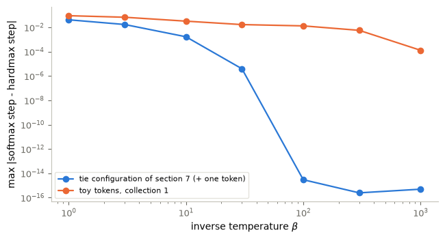
Figure (softmax). One softmax attention step against one hardmax step (\(A=I\), \(\alpha=0.1\)), as the inverse temperature \(\beta\) grows, for a configuration with an exact three-way tie and for the first collection of toy tokens.
Interpretation. The deviation decays like \(e^{-\beta g}\), with \(g\) the smallest gap between a row’s maximum and its next score (printed). It is negligible once \(\beta g\) is a few tens. With the tie, softmax converges to the average over the three tied tokens, the hardmax rule. A configuration with tiny gaps would need a very large \(\beta\): softmax and hardmax dynamics can differ substantially over many layers.
12. Sentiment analysis and prompt engineering
The hardmax model has been applied to a supervised task: classify IMDb movie reviews as positive or negative (Alcalde, Fantuzzi and Zuazua, 2025). A review of \(n\) words, each a canonical basis vector of \(\mathbb R^W\) (\(W\) the vocabulary size), passes through three steps: 1. an encoder \(Z^0=XE\) with a trainable \(E\in\mathbb R^{W\times d}\); 2. the transformer \(Z^K=\mathcal T_{A,\alpha}(Z^0)\); 3. a decoder \(\hat y=\sigma\big(\frac1n\mathbf 1^\top Z^Kv+b\big)\), a logistic readout of the average token.
With \(A=I\) fixed and \(E\), \(v\), \(b\), \(\alpha\) trained, the model admits a complete reading: the encoder places relevant words (those conveying sentiment) as leaders; the transformer filters out irrelevant words by clustering them to the leaders; the decoder divides \(\mathbb R^d\) into two half-spaces, one per sentiment.
Prompt engineering then changes a few words of a review classified as negative, e.g. “worst” → “best”, “lamest” → “greatest”, until it is classified as positive — mathematically, modifying words to change the clustering pattern. These are interpretations of a trained model, reported in the cited work; we have not reproduced the experiment, and no data set is used in §§7–12. The leader/follower picture of this notebook is what gives them a precise meaning.
13. Modern self-attention
The core operations in §§1–5 also appear in larger models, alongside additional architectural and implementation choices. The 2017 base model had \(65\)M parameters and was trained in twelve hours on eight GPUs. BERT-base has \(110\)M, GPT-2 has \(1.5\)B, and GPT-3 has \(175\)B spread over \(96\) layers with \(d_m = 12288\) and \(96\) heads — at \(2\) bytes per parameter in float16 the weights alone occupy about \(350\) GB, so the model cannot be held on one \(80\) GB accelerator and requires multiple accelerators just to store those weights; Llama 3.1 405B needs roughly \(810\) GB at the same precision. Our TinyBERT has about \(10^5\) parameters, some six orders of magnitude less, and is the same six equations.
Two costs then dominate engineering. First, memory at inference: a decoder caches \(K\) and \(V\) for every past token, \(2 \cdot L \cdot d_m\) values per token, which for GPT-3 is \(\approx 4.7\) MB per token, or about \(10\) GB for a full \(2048\)-token context — per sequence. This is why grouped-query and multi-query attention, which share keys and values across heads, are now standard. Second, the \(\mathcal{O}(n^2)\) itself: context windows have gone from \(2048\) tokens to \(10^5\)–\(10^6\), where a single head’s attention matrix would have \(10^{12}\) entries. FlashAttention (Dao et al., 2022) does not reduce the arithmetic but tiles the computation so the \(n \times n\) matrix is never written to memory, which is what made long contexts practical; sliding-window and sparse patterns, linear-attention and state-space models (Mamba), and mixture-of-experts layers for growing parameters without growing compute all attack the same two walls.
The mathematically interesting point is that scale did not require a new mechanism. A learned, asymmetric kernel smoother, stacked in a residual stream — that is still all it is.
14. Control ↔︎ ML
- Residual updates. MATHEMATICAL ANALOGY with residual networks. Attention and feed-forward blocks are residual steps — one Euler step each — but the attention step depends on all tokens: it is the update of an interacting-particle system, not of \(n\) independent copies of one system.
- State-dependent averaging = consensus dynamics. MATHEMATICAL ANALOGY. Each token moves towards an average of others chosen by the current configuration, as agents do in consensus and flocking models. Here the convex hull shrinks, leaders are fixed points, and clusters form.
- Clustering and classification. FORWARD CONNECTION with classification as simultaneous control, and §12. In the sentiment-analysis reading, the encoder places relevant words as leaders, attention clusters the others around them, and a half-space readout decides the label.
Key takeaways
- Self-attention forms data-dependent convex combinations of value vectors: a learned Nadaraya–Watson kernel smoother, at cost \(O(n^2)\).
- Scaling by \(1/\sqrt{d_a}\) keeps attention logits controlled; multiple heads learn different low-rank comparisons; positional information must be injected, since attention is permutation-equivariant.
- The residual stream makes a deep transformer a discretized flow on a cloud of interacting particles (Euler steps, now coupled).
- Masked-token prediction trains the encoder to combine information from both sides of a hole; a
[MASK]after the context turns it into a next-token model, and the chain rule turns that into a generator. - Hardmax attention averages over all maximizers; with \(V=\alpha I\) and the normalization by \(1+\alpha\), each step is a convex combination with step \(\alpha/(1+\alpha)\).
- Tokens stay in the convex hull of the initial tokens; leaders never move and stay leaders; a follower of a fixed leader approaches it at the rate \((1+\alpha)^{-k}\).
- For nonzero, distinct tokens and \(A\) symmetric positive definite, every token converges to a leader or to a projection of the origin onto a face of the leaders’ polytope. The theorem gives no rate.
- Finite runs in floating point show the clustering, and also artefacts such as followers that become exactly equal to their leaders. They illustrate the theorem; they do not prove it.
15. Exercises
★ conceptual · ★★ mathematical · ★★★ computational
- Scaling. ★★★ Remove the factor \(1/\sqrt{d_a}\) from
TinyBERT’s attention and compare the attention entropy and the held-out accuracy after retraining. - Order. ★★★ Remove the positional encoding from
TinyBERT, retrain, and generate. Which features of the text survive? - Heads. ★★★ Train with one head and four heads at the same model width. Compare held-out accuracy and the attention maps.
- Next character. ★★★ Delete the line that always hides the last character, retrain, and compare the generated text.
- Who leads? ★ Take \(A=I\). (a) Show that a token of largest norm, if unique, is a leader. (b) Give three tokens in \(\mathbb R^2\) with two leaders, one of which does not have the largest norm. (c) Is a token in the interior of the convex hull of the others ever a leader?
- The normalization. ★★ (a) Starting from the unnormalized layer with \(V=\alpha I\), derive the boxed update of §7 and its two forms. (b) What happens to a leader over \(K\) layers without the division by \(1+\alpha\)? (c) Verify numerically on a collection of toy tokens that the normalized layer coincides with
hardmax_step. - Why nonzero and distinct? ★★ (a) Show that the token \(z_i=0\) attends to every token, and compute its next position. (b) Show that two identical tokens attend to the same set and remain identical forever. (c) Explain how each fact interferes with the statement “the leaders are the vertices of \(\mathcal K\)” of the theorem.
- A different attention matrix. ★★ Take \(A=\mathrm{diag}(1,9)\) and the first collection of toy tokens. (a) Compute the initial leaders and compare with \(A=I\). (b) Run 400 layers and count the clusters. (c) Interpret: what does \(A\) change in the geometry of “who attends to whom”?
- Planted leaders. ★★★ Design an initial configuration with three planted leaders, the points of radius \(2\) at angles \(90^\circ\), \(210^\circ\) and \(330^\circ\), and ten other tokens drawn from a small disc of radius \(0.5\) around the origin, deterministically (for instance on a spiral). (a) Check that exactly the three planted tokens are leaders. (b) Predict, from the scores, which leader each of the ten tokens will follow, and verify after 400 layers. (c) Can you place an additional token so that it rests at the projection of the origin onto an edge of the triangle?
- How many layers? ★★★ (a) Using the follower rate of §8, how many layers are needed for a follower to get within \(10^{-6}\) of its leader from an initial distance \(1\), for \(\alpha=0.1\) and for \(\alpha=1\)? (b) Check the prediction for \(\alpha=0.1\) on the residual curves of §10, taking into account that a token may change its attended set before following a fixed leader. (c) Why can no statement of this kind be uniform over all configurations?
# TODO: student exercise (Exercise 9)
# Return a (13, 2) array: three planted leaders first, then ten tokens in the disc of radius 0.5.

def planted_tokens():
    ...  # your code here
    return None
Where are we going?
With many tokens, it is natural to stop following each one and to follow their distribution instead. Notebook 16 does this for neural ODEs: a flow transports a probability density, the control is chosen to transport one distribution to another, and the same fields learn dynamics from trajectory data.
References
- A. Vaswani, N. Shazeer, N. Parmar, J. Uszkoreit, L. Jones, A. N. Gomez, Ł. Kaiser, I. Polosukhin, Attention is all you need, NeurIPS 2017.
- J. Devlin, M.-W. Chang, K. Lee, K. Toutanova, BERT: pre-training of deep bidirectional transformers for language understanding, NAACL 2019.
- A. Karpathy, The unreasonable effectiveness of recurrent neural networks, 2015 — the source of Tiny Shakespeare; and nanoGPT, a decoder-only counterpart to §6.
- A. Rush, The annotated transformer, 2018.
- Y.-H. Tsai, S. Bai, M. Yamada, L.-P. Morency, R. Salakhutdinov, Transformer dissection: a unified understanding of transformer’s attention via the lens of kernel, EMNLP 2019.
- R. Xiong et al., On layer normalization in the transformer architecture, ICML 2020.
- J. Su, Y. Lu, S. Pan, A. Murtadha, B. Wen, Y. Liu, RoFormer: enhanced transformer with rotary position embedding, Neurocomputing, 2024.
- T. Dao, D. Y. Fu, S. Ermon, A. Rudra, C. Ré, FlashAttention: fast and memory-efficient exact attention with IO-awareness, NeurIPS 2022.
- N. Elhage et al., A mathematical framework for transformer circuits, Anthropic, 2021.
- B. Geshkovski, C. Letrouit, Y. Polyanskiy, P. Rigollet, A mathematical perspective on transformers, Bulletin of the AMS, 2025 — attention as an interacting particle system.
- A. Alcalde, G. Fantuzzi, E. Zuazua, Clustering in pure-attention hardmax transformers and its role in sentiment analysis, SIAM Journal on Mathematics of Data Science 7 (2025); arXiv:2407.01602.