%matplotlib inline
import numpy as np
import torch
import matplotlib.pyplot as plt
import plotting as P           # the course palette, the house style, and the figure helpers

torch.manual_seed(0);02 — Linear Control Systems and the Kalman Rank Condition
Mathematical Foundations of Control and Machine Learning — Winter 2026
Central question. When can a linear system with few controls be steered between arbitrary states?
This notebook answers the controllability question completely for linear, finite-dimensional systems: the Kalman rank condition decides it, and the controllability Gramian turns the answer into an explicit steering control.
Table of Contents
- Linear control systems — variation of constants, exact controllability, the spring–mass–damper
- Two first examples — an uncontrollable system; “draw a curve, read off the control”
- The reachable set — an affine subspace described by one matrix, with the complete proof
- The Kalman rank condition — the theorem as a corollary, the near-uncontrollable family, the rank block by block
- Genericity, robustness and numerical rank — most systems are controllable, the chain of integrators
- The controllability Gramian and an explicit steering control — the matrix that measures control, formula (G), and an animation
- Quantitative controllability — the near-uncontrollable family
- Control ↔︎ ML and beyond linear systems — one system or many, Nelson’s car
- Exercises
# RK4 integrator for x' = f(t, x) along the time grid ts
def odeint(f, x0, ts):
    xs = [x0]
    for t, t1 in zip(ts[:-1], ts[1:]):
        x, h = xs[-1], t1 - t
        k1 = f(t, x)
        k2 = f(t + h / 2, x + h / 2 * k1)
        k3 = f(t + h / 2, x + h / 2 * k2)
        k4 = f(t + h, x + h * k3)
        xs.append(x + h / 6 * (k1 + 2 * k2 + 2 * k3 + k4))
    return torch.stack(xs)

def lti(A, B, u):
    """Right-hand side of x' = Ax + Bu, with u an open-loop control u(t) -> R^m."""
    return lambda t, x: A @ x + B @ u(t)

def l2_effort(u, ts):
    """The L2 norm (∫|u|² dt)^{1/2} of a control along the grid ts."""
    vals = torch.stack([u(s) for s in ts])
    return float(torch.sqrt(torch.trapezoid((vals ** 2).sum(-1), ts)))
Where are we?
Three questions organize control theory: controllability (can we reach a target?), optimal control (which control is best?) and stabilization (is there a rule that drives the system to rest?). This notebook answers the first question completely for linear, finite-dimensional systems. It is the setting where everything is explicit, and every later setting is measured against it.
1. Linear control systems
Let \(n,m\ge1\) and \(T>0\). We consider
\[ x'(t)=Ax(t)+Bu(t),\quad t\in(0,T),\qquad x(0)=x^0, \]
with \(A\in\mathbb R^{n\times n}\), \(B\in\mathbb R^{n\times m}\) and \(x^0\in\mathbb R^n\). The state \(x(t)\) has \(n\) components and the control \(u(t)\) has \(m\). In practice \(m\le n\), and often \(m\ll n\): the most desirable situation is to control the system with as few controls as possible.
Example (the spring–mass–damper). A mass \(m_0\) is attached to a spring of stiffness \(k\) and a damper of coefficient \(c\). We measure displacement \(q\) from equilibrium and apply a force \(u(t)\). Newton’s second law reads \(m_0\ddot q = -kq - c\dot q + u\). Writing \(x = (x_1, x_2)^\top\) with \(x_1 = q\) the position and \(x_2 = \dot q\) the velocity turns one second-order equation into two first-order ones: \[ \begin{bmatrix} \dot x_1 \\ \dot x_2 \end{bmatrix} = \underbrace{\begin{bmatrix} 0 & 1 \\ -\tfrac{k}{m_0} & -\tfrac{c}{m_0} \end{bmatrix}}_{A} \begin{bmatrix} x_1 \\ x_2 \end{bmatrix} + \underbrace{\begin{bmatrix} 0 \\ \tfrac{1}{m_0} \end{bmatrix}}_{B} u . \] With \(m_0=k=1\) and no damper, \(c=0\), this is the harmonic oscillator \(x_1''+x_1=u\).
Variation of constants. Multiply the equation by \(e^{-At}\): \[ \big(e^{-At}x(t)\big)'=e^{-At}\big(x'(t)-Ax(t)\big)=e^{-At}Bu(t). \] Integrating from \(0\) to \(t\) and multiplying by \(e^{At}\) gives
\[ x(t)=e^{At}x^0+\int_0^te^{A(t-s)}Bu(s)\,ds . \tag{1} \]
Definition (exact controllability). The system is exactly controllable in time \(T\) if for every \(x^0,x^1\in\mathbb R^n\) there is \(u\in L^2(0,T;\mathbb R^m)\) such that the solution satisfies \(x(T)=x^1\).
The control process drives the solution from \(x^0\) to \(x^1\) in time \(T\), by acting on the system through \(u\).
fig, ax = P.panels(figsize=(6.2, 2.8))
P.spring_mass_damper(ax, pos=1.1)
plt.show()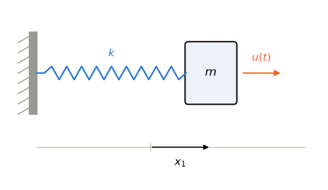
2. Two first examples
Example 1: an uncontrollable system. With \(A=\begin{pmatrix}1&0\\0&1\end{pmatrix}\) and \(B=\begin{pmatrix}1\\0\end{pmatrix}\), the system reads \[ x_1'=x_1+u,\qquad x_2'=x_2\ \ \Longrightarrow\ \ x_2(t)=x_2^0e^t . \] The control does not act on the second component, which is completely determined by its initial value, so the system is not controllable.
Example 2: the harmonic oscillator is controllable. For \(x_1''+x_1=u\), a direct argument works. Choose any smooth curve \(x_1(t)\) with the prescribed position and velocity at \(t=0\) and at \(t=T\), and define the control afterwards: \[ u(t)=x_1''(t)+x_1(t). \] By construction this \(u\) steers the system between the prescribed states. For instance, to stop the oscillator, from \(x^0=(1,0)\) to \(x^1=(0,0)\) at \(T=5\), the cubic \(x_1(t)=1-3(t/T)^2+2(t/T)^3\) has the right boundary values.
A = torch.tensor([[0.0, 1.0], [-1.0, 0.0]])            # the harmonic oscillator: x1'' + x1 = u
B = torch.tensor([[0.0], [1.0]])
T = 5.0
x0 = torch.tensor([1.0, 0.0])                          # displaced, at rest
x1 = torch.tensor([0.0, 0.0])                          # at rest at the origin
ts = torch.linspace(0, T, 2001)

# "Draw a curve, read off the control": cubic with x1(0)=1, x1'(0)=0, x1(T)=0, x1'(T)=0.
curve = lambda s: 1 - 3 * (s / T) ** 2 + 2 * (s / T) ** 3
curve_dd = lambda s: -6 / T ** 2 + 12 * s / T ** 3
u_curve = lambda s: (curve_dd(s) + curve(s)).reshape(1)          # u = x1'' + x1

x_curve = odeint(lti(A, B, u_curve), x0, ts)
print("x(T) with the curve control:", x_curve[-1].numpy().round(6),
      "   L2 effort:", round(l2_effort(u_curve, ts), 4))
x(T) with the curve control: [ 0. -0.] L2 effort: 1.21373. The reachable set
Is the control obtained from the cubic the only control that stops the oscillator? No: any other curve with the same boundary values gives another control. To organize all the possibilities, we collect the states that can be reached:
\[ \mathcal R(T,x^0)=\big\{x(T)\;:\;x\text{ solves (1) with some }u\in L^2(0,T;\mathbb R^m)\big\}. \]
Exact controllability means \(\mathcal R(T,x^0)=\mathbb R^n\) for every \(x^0\).
By (1), \(x(T)=e^{AT}x^0+L_Tu\), with the linear input-to-state map \[ L_T:L^2(0,T;\mathbb R^m)\to\mathbb R^n,\qquad L_Tu=\int_0^Te^{A(T-s)}Bu(s)\,ds . \] So \(\mathcal R(T,x^0)=e^{AT}x^0+\operatorname{Range}L_T\) is an affine subspace: the free evolution of \(x^0\), plus everything the control can add. The key fact is that the directions the control can add are described by a single matrix.
Definition (Kalman matrix). \(\mathcal K(A,B)=[\,B,\;AB,\;A^2B,\;\dots,\;A^{n-1}B\,]\in\mathbb R^{n\times nm}\).
Theorem 1 (reachable set). Assumptions: \(A\in\mathbb R^{n\times n}\), \(B\in\mathbb R^{n\times m}\), \(T>0\).
Conclusion: \(\operatorname{Range}L_T=\operatorname{Range}\mathcal K(A,B)\). Hence \[\mathcal R(T,x^0)=e^{AT}x^0+\operatorname{Range}\mathcal K(A,B)\qquad\text{for every }x^0\text{ and every }T>0 .\]
Interpretation: the reachable set is an affine subspace whose direction does not depend on \(T\) or \(x^0\); only its offset \(e^{AT}x^0\) does.
Proof of “\(\subseteq\)” (Cayley–Hamilton). By the Cayley–Hamilton theorem, \(A\) satisfies its characteristic polynomial, so \(A^n\), and inductively every \(A^j\) with \(j\ge n\), is a linear combination of \(I,A,\dots,A^{n-1}\). Hence every column of every \(A^jB\) lies in \(\operatorname{Range}\mathcal K\). The power series \(e^{A(T-s)}B=\sum_{j\ge0}\frac{(T-s)^j}{j!}A^jB\) converges, and \(\operatorname{Range}\mathcal K\) is closed, so each column of \(e^{A(T-s)}B\) lies in \(\operatorname{Range}\mathcal K\). Integrating against \(u(s)\) keeps us there: \(L_Tu\in\operatorname{Range}\mathcal K\).
Proof of “\(\supseteq\)” (all derivatives vanish). Both ranges are subspaces of \(\mathbb R^n\), so it suffices to show that every \(v\) orthogonal to \(\operatorname{Range}L_T\) is orthogonal to \(\operatorname{Range}\mathcal K\). Let \(v\perp\operatorname{Range}L_T\). For every control, \[ 0=\langle v,L_Tu\rangle=\int_0^T\big\langle B^*e^{A^*(T-s)}v,\,u(s)\big\rangle\,ds . \] Choosing \(u(s)=B^*e^{A^*(T-s)}v\) gives \(\int_0^T|B^*e^{A^*(T-s)}v|^2\,ds=0\). The integrand is continuous, so \[ g(s):=B^*e^{A^*(T-s)}v=0\qquad\text{for all }s\in[0,T]. \] The function \(g\) is smooth and vanishes identically, so all its derivatives vanish. At \(s=T\), \(g^{(j)}(T)=(-1)^jB^*(A^*)^jv=0\) for all \(j\ge0\). In other words, \(v\) is orthogonal to every column of \(A^jB\), hence to \(\operatorname{Range}\mathcal K\). \(\square\)
4. The Kalman rank condition
Theorem 1 reduces controllability to linear algebra: whatever the horizon, the directions the control can add are exactly \(\operatorname{Range}\mathcal K(A,B)\). The classical result of R. E. Kalman follows at once.
Theorem 2 (Kalman, 1960). Assumptions: \(A\in\mathbb R^{n\times n}\), \(B\in\mathbb R^{n\times m}\).
Conclusion: the system \(x'=Ax+Bu\) is exactly controllable in some time \(T>0\) if and only if \[\operatorname{rank}\,[\,B,\,AB,\,\dots,\,A^{n-1}B\,]=n .\] Consequently, if it is controllable in some time \(T>0\), it is controllable in every time \(T>0\).
Proof. By Theorem 1, \(\mathcal R(T,x^0)=e^{AT}x^0+\operatorname{Range}\mathcal K\). This affine subspace is all of \(\mathbb R^n\) if and only if \(\operatorname{Range}\mathcal K=\mathbb R^n\), that is, if and only if \(\operatorname{rank}\mathcal K=n\). The condition does not involve \(T\). \(\square\)
Example. An uncontrollable example in three dimensions The near-uncontrollable family, studied quantitatively in §7, is \[ A=\begin{pmatrix}0&1&0\\-1&0&0\\0&0&-1\end{pmatrix},\qquad B_\varepsilon=\begin{pmatrix}0\\1\\\varepsilon\end{pmatrix}: \] an oscillator coupled to a decaying mode \(x_3'=-x_3+\varepsilon u\), which the actuator reaches with strength \(\varepsilon\). For \(\varepsilon=0\) the actuator acts only on the oscillator, and \(\operatorname{Range}\mathcal K=\{x_3=0\}\). From \(x^0=(0,0,1)\) the reachable set is therefore the horizontal plane \(\{x_3=e^{-T}\}\), whatever the control.
def kalman(A, B):
    """Kalman matrix [B | AB | ... | A^{n-1}B]."""
    cols = [B]
    for _ in range(A.shape[0] - 1):
        cols.append(A @ cols[-1])
    return torch.cat(cols, dim=1)

def num_rank(M):
    """Numerical rank and singular values: how many s_i exceed max(shape)·eps_mach·s_max."""
    s = torch.linalg.svdvals(M)
    return int((s > max(M.shape) * torch.finfo(M.dtype).eps * s[0]).sum()), s

def family(eps):
    A = torch.tensor([[0.0, 1.0, 0.0], [-1.0, 0.0, 0.0], [0.0, 0.0, -1.0]])
    return A, torch.tensor([[0.0], [1.0], [eps]])

# Numerical rank of [B], [B, AB], [B, AB, A²B] for the near-uncontrollable family
print(f"{'eps':>4} {'[B]':>4} {'[B,AB]':>7} {'[B,AB,A²B]':>11}   singular values of K")
for eps in (0.0, 0.1, 0.3):
    K = kalman(*family(eps))
    ranks = [num_rank(K[:, :k])[0] for k in (1, 2, 3)]
    s = "  ".join(f"{float(x):.4f}" for x in num_rank(K)[1])
    print(f"{eps:>4} {ranks[0]:>4} {ranks[1]:>7} {ranks[2]:>11}   {s}")
eps [B] [B,AB] [B,AB,A²B] singular values of K
0.0 1 2 2 1.4142 1.0000 0.0000
0.1 1 2 3 1.4142 1.0051 0.1407
0.3 1 2 3 1.4142 1.0524 0.40325. Genericity, robustness and numerical rank
Controllable pairs are open and dense. Controllability fails exactly when all \(n\times n\) minors of \(\mathcal K(A,B)\) vanish. Each minor is a polynomial in the entries of \((A,B)\). The set where finitely many polynomials vanish, not all of them identically zero, is closed and has empty interior. So controllability is robust: it survives small perturbations of \(A\) and \(B\). And it is generic: most systems are controllable, and an arbitrarily small perturbation makes an uncontrollable pair controllable.
Cost estimate. When controllability holds, there is a control with \(\|u\|_{L^2(0,T)}\le C\,|e^{AT}x^0-x^1|\), where \(C\) depends on \((A,B,T)\). The size of \(C\) is the quantitative side of controllability. The Gramian of §6 makes it computable.
Example. The typical example where every block is needed is \[ x^{(n)}=u. \] For the state \((x,x',\dots,x^{(n-1)})\), \[A=\begin{pmatrix}0&1&&\\&0&\ddots&\\&&\ddots&1\\&&&0\end{pmatrix},\qquad B=e_n,\qquad\text{so}\qquad B=e_n,\quad AB=e_{n-1},\quad A^2B=e_{n-2},\quad\dots,\quad A^{n-1}B=e_1 .\] Each block contributes exactly one new direction, and the rank reaches \(n\) only with \(A^{n-1}B\): the control acts directly on \(x^{(n-1)}\), on \(x^{(n-2)}\) after one integration, and on the position \(x\) only after \(n-1\) of them.
6. The controllability Gramian and an explicit steering control
The proof of Theorem 1 used the control \(u(s)=B^*e^{A^*(T-s)}v\). Applying \(L_T\) to controls of this form produces a matrix.
Definition (controllability Gramian). \(\displaystyle\mathcal G_T=\int_0^Te^{A(T-s)}BB^*e^{A^*(T-s)}\,ds\in\mathbb R^{n\times n}.\)
Proposition 3 (properties of the Gramian). 1. \(\mathcal G_T\) is symmetric and positive semidefinite: \(v^*\mathcal G_Tv=\int_0^T|B^*e^{A^*(T-s)}v|^2ds\ge0\). 2. \(\ker\mathcal G_T=(\operatorname{Range}\mathcal K)^\perp\). 3. \(\mathcal G_T\) is invertible if and only if \(\operatorname{rank}\mathcal K=n\), that is, if and only if the system is controllable. 4. \(L_T\big(B^*e^{A^*(T-\cdot)}c\big)=\mathcal G_Tc\) for every \(c\in\mathbb R^n\).
Proof. (1) Symmetry is clear from the formula, and the identity follows from \(v^*e^{A(T-s)}BB^*e^{A^*(T-s)}v=|B^*e^{A^*(T-s)}v|^2\).
\(\mathcal G_Tv=0\) implies \(v^*\mathcal G_Tv=0\), hence \(g(s)=B^*e^{A^*(T-s)}v\equiv0\), and the derivative argument in the proof of Theorem 1 gives \(v\perp\operatorname{Range}\mathcal K\). Conversely, if \(v\perp\operatorname{Range}\mathcal K\), then \(v\) is orthogonal to every column of \(e^{A(T-s)}B\) by the Cayley–Hamilton step of Theorem 1. So \(g\equiv0\), and \(\mathcal G_Tv=\int_0^Te^{A(T-s)}B\,g(s)\,ds=0\).
follows from (2) and Theorem 2. (4) is the definition of \(L_T\) applied to \(u(s)=B^*e^{A^*(T-s)}c\). \(\square\)
If the system is controllable, property (4) tells us how to reach any target. We want \(L_Tu=x^1-e^{AT}x^0\); try \(u=B^*e^{A^*(T-\cdot)}c\) and solve \(\mathcal G_Tc=x^1-e^{AT}x^0\):
\[ \boxed{\;u(t)=B^*e^{A^*(T-t)}\,\mathcal G_T^{-1}\big(x^1-e^{AT}x^0\big).\;} \tag{G} \]
Verification. By (1) and the definition of \(\mathcal G_T\), \[ x(T)=e^{AT}x^0+\int_0^Te^{A(T-s)}BB^*e^{A^*(T-s)}\,ds\;\mathcal G_T^{-1}\big(x^1-e^{AT}x^0\big)=e^{AT}x^0+\big(x^1-e^{AT}x^0\big)=x^1 . \]
We now compute (G) for the harmonic oscillator, stopping the oscillator from \(x^0=(1,0)\) at \(T=5\), as in §2, and compare it with the free motion of the oscillator.
def gramian(A, B, T, n_quad=400):
    """G_T = ∫_0^T e^{A(T-s)} B Bᵀ e^{Aᵀ(T-s)} ds, by the trapezoid rule (τ = T - s)."""
    taus = torch.linspace(0, T, n_quad + 1)
    integrand = torch.stack([(E := torch.matrix_exp(A * tau)) @ B @ B.T @ E.T for tau in taus])
    return torch.trapezoid(integrand, taus, dim=0)

class GramianControl:
    """The steering control (G): u(t) = Bᵀ e^{Aᵀ(T-t)} G_T⁻¹ (x¹ - e^{AT} x⁰)."""
    def __init__(self, A, B, x0, x1, T):
        self.A, self.B, self.T = A, B, T
        self.G = gramian(A, B, T)
        self.d = x1 - torch.matrix_exp(A * T) @ x0
        self.c = torch.linalg.solve(self.G, self.d)
    def __call__(self, t):
        return self.B.T @ torch.matrix_exp(self.A.T * (self.T - t)) @ self.c
    def effort(self):                                  # (∫|u|² dt)^{1/2} = (dᵀ G_T⁻¹ d)^{1/2}
        return float(torch.sqrt(self.d @ self.c))

G = gramian(A, B, T)
print("Kalman matrix K = [B, AB] =\n", kalman(A, B).numpy())
print("Gramian G_T =\n", G.numpy().round(5))
print("symmetric:", bool(torch.allclose(G, G.T)), "   eigenvalues:",
      np.round(torch.linalg.eigvalsh(G).numpy(), 5))

u_G = GramianControl(A, B, x0, x1, T)
x_G = odeint(lti(A, B, u_G), x0, ts)
x_free = odeint(lti(A, B, lambda t: torch.zeros(1)), x0, ts)
print(f"\n|x(T) - x1| with the Gramian control (G): {float((x_G[-1] - x1).norm()):.1e}")

idx = torch.arange(0, len(ts), 40)                     # ~50 frames
pf, pc = x_free[idx, 0].numpy(), x_G[idx, 0].numpy()

fig, (axm, axt) = P.panels(1, 2, ratios=[1.1, 1], figsize=(6.4, 4.6))
up_free = P.spring_mass_artist(axm, 0.8, P.GREY, "no control")
up_ctrl = P.spring_mass_artist(axm, -0.8, P.BLUE, "control (G)")
axm.plot(0.0, -0.8, "*", color=P.ORANGE, ms=14, zorder=0)
P.label(axm, xlim=(-3.0, 2.3), ylim=(-1.8, 1.8), equal=True, off=True)

axt.plot(ts, x_free[:, 0], color=P.GREY, lw=1.2)
axt.plot(ts, x_G[:, 0], color=P.BLUE, lw=1.5)
axt.plot(T, 0.0, "*", color=P.ORANGE, ms=12)
cursor = axt.axvline(0, color=P.ORANGE, lw=1)
P.label(axt, "$t$", "$x_1$", xlim=(0, T))

def update(i):
    up_free(pf[i]); up_ctrl(pc[i]); cursor.set_xdata([ts[idx[i]]] * 2)

P.animate(fig, update, len(idx), interval=60)
Kalman matrix K = [B, AB] =
[[0. 1.]
[1. 0.]]
Gramian G_T =
[[2.63599 0.45974]
[0.45974 2.364 ]]
symmetric: True eigenvalues: [2.02057 2.97943]
|x(T) - x1| with the Gramian control (G): 9.4e-067. Quantitative controllability: the near-uncontrollable family
The Kalman condition is a yes/no answer, and a “yes” can hide very different behaviours. We measure them on the near-uncontrollable family of §4: \[ A=\begin{pmatrix}0&1&0\\-1&0&0\\0&0&-1\end{pmatrix},\qquad B_\varepsilon=\begin{pmatrix}0\\1\\\varepsilon\end{pmatrix}. \] A direct computation gives \(\det\mathcal K(A,B_\varepsilon)=-2\varepsilon\), so the pair is controllable for every \(\varepsilon\ne0\).
Using (G), the \(L^2\) effort of that control for a displacement \(d=x^1-e^{AT}x^0\) is \(\big(d^*\mathcal G_T^{-1}d\big)^{1/2}\), so its energy is \(\int_0^T|u|^2\,dt=d^*\mathcal G_T^{-1}d\). We steer from \(x^0=0\) to the weak mode \(e_3\). As \(\varepsilon\to0\), how much energy does this need?
Code and plot. Sweep \(\varepsilon\) from \(10^{-3}\) to \(1\) on log–log axes.
epsilons = np.logspace(-3, 0, 13)
target = torch.tensor([0.0, 0.0, 1.0])                 # the weak mode e_3

# energy ∫|u|² dt = dᵀ G_T⁻¹ d of the control (G) that steers x0 = 0 to the target
energy = [GramianControl(*family(float(eps)), torch.zeros(3), target, T).effort() ** 2
          for eps in epsilons]

fig, ax = P.panels(size=(4.4, 3.4))
ax.loglog(epsilons, energy, "o-", color=P.ORANGE)
P.label(ax, r"actuator strength $\varepsilon$", r"energy $\int_0^T|u|^2\,dt$")
plt.show()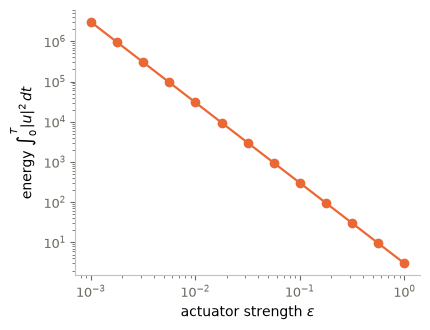
8. Control ↔︎ ML and beyond linear systems
Classical controllability asks whether one system can be steered by its control: the Kalman theorem answers how many states \(n\) a few controls \(m\) can handle. In the machine-learning part of the course the question is turned around. Supervised learning is read as simultaneous (ensemble) control: many trajectories, one per data point, steered by one shared control, the parameters of the network. The rank argument of this notebook does not apply there, and different, geometric constructions are needed.
For nonlinear systems, controllability can come from combining motions rather than from a rank test on \((A,B)\). The classical illustration is Nelson’s car: two controls, steering and driving, suffice to control a four-dimensional state, consisting of the position, the orientation of the car and the angle of the wheels — the mathematics of the parking manoeuvre. Behind it is the theory of Lie brackets (see Sontag or Coron).
Key takeaways
- Variation of constants: \(x(T)=e^{AT}x^0+L_Tu\) with \(L_Tu=\int_0^Te^{A(T-s)}Bu(s)\,ds\).
- Reachable set: \(\mathcal R(T,x^0)=e^{AT}x^0+\operatorname{Range}\mathcal K(A,B)\), an affine subspace whose direction does not depend on \(T\).
- Kalman: controllable ⟺ \(\operatorname{rank}[B,AB,\dots,A^{n-1}B]=n\); and then controllable in every time \(T>0\).
- The proof of Theorem 1 uses Cayley–Hamilton (“\(\subseteq\)”) and the vanishing of all derivatives of \(B^*e^{A^*(T-s)}v\) at \(s=T\) (“\(\supseteq\)”); Kalman’s theorem is a corollary. The rank of \([B,AB,\dots,A^kB]\) grows until it stalls and then stays; the chain of integrators \(x^{(n)}=u\) needs all \(n\) blocks.
- Gramian: \(\mathcal G_T\) is symmetric, positive semidefinite, with \(\ker\mathcal G_T=(\operatorname{Range}\mathcal K)^\perp\); it is invertible iff the system is controllable.
- Formula (G) steers \(x^0\) to \(x^1\) exactly, with effort \(\big(d^*\mathcal G_T^{-1}d\big)^{1/2}\) for the displacement \(d=x^1-e^{AT}x^0\).
- The rank is algebraic; singular values and Gramian eigenvalues measure how hard control is, direction by direction.
9. Exercises
★ conceptual · ★★ mathematical · ★★★ computational
- Predict the rank. ★ Without computing, predict whether each pair is controllable, then check with the
kalmanandnum_rankcode above: (a) the double integrator \(A=\begin{pmatrix}0&1\\0&0\end{pmatrix}\), \(B=\begin{pmatrix}0\\1\end{pmatrix}\); (b) \(A=\operatorname{diag}(1,2)\), \(B=\begin{pmatrix}1\\1\end{pmatrix}\); (c) \(A=I_2\), \(B=\begin{pmatrix}1\\1\end{pmatrix}\); (d) \(A=\operatorname{diag}(1,2)\), \(B=\begin{pmatrix}1\\0\end{pmatrix}\). - Scalar equations of order \(n\). ★★ Write \(x^{(n)}+a_{n-1}x^{(n-1)}+\dots+a_1x'+a_0x=u\) as a first-order system for \((x,x',\dots,x^{(n-1)})\) (companion form). Show that \(\mathcal K(A,B)\) is triangular with nonzero diagonal, so the system is controllable with a single control, whatever the coefficients. For \(a_j=0\) this is the chain of integrators of §5.
- Reachable sets. ★★ (a) For Example 1 (\(A=I_2\), \(B=e_1\)), describe \(\mathcal R(T,x^0)\) explicitly as a set in the plane, and say how it moves as \(T\) grows. (b) For a general pair, show that \(\mathcal R(T,x^0)=\mathcal R(T,y^0)\) if and only if \(e^{AT}(x^0-y^0)\in\operatorname{Range}\mathcal K\), and interpret this for the near-uncontrollable family at \(\varepsilon=0\).
- The rank, block by block. ★★ Let \(r_k=\operatorname{rank}[B,AB,\dots,A^kB]\). (a) Prove that the rank stalls for good: if \(r_{k+1}=r_k\) then \(r_j=r_k\) for every \(j\ge k\). (b) Deduce, without Cayley–Hamilton, that \(\operatorname{Range}\mathcal K(A,B)\) is the smallest \(A\)-invariant subspace containing the columns of \(B\), and that \(\operatorname{span}\{A^jB\text{ columns}:j\ge0\}=\operatorname{Range}\mathcal K\). (c) Show that if \(\operatorname{rank}\mathcal K<n\), there is \(v\ne0\) with \(v^*e^{tA}B=0\) for all \(t\in\mathbb R\), and explain why this makes \(\langle v,x(t)\rangle\) independent of the control.
- The Gramian grows with \(T\). ★★ (a) Show that \(T\mapsto\mathcal G_T\) is non-decreasing: \(\mathcal G_{T'}-\mathcal G_T\) is positive semidefinite for \(T'>T\). (b) Deduce that \(\lambda_{\min}(\mathcal G_T)\) is non-decreasing in \(T\). (c) Using the effort formula \(\big(d^*\mathcal G_T^{-1}d\big)^{1/2}\) of §7, show that the control (G) needs no more effort for a longer horizon, for the same displacement \(d\). Why is this the same \(d\) for the harmonic oscillator only when \(x^0=0\)?
- Two almost identical oscillators. ★★★ Two oscillators with frequencies \(1\) and \(1+\delta\) are driven by the same input: \(A=\operatorname{diag}(A_{\rm osc},A_{1+\delta})\) with \(A_\omega=\begin{pmatrix}0&1\\-\omega^2&0\end{pmatrix}\), and \(B=(0,1,0,1)^\top\). For \(\delta=0\) the pair is uncontrollable. For \(\delta\in\{1,0.3,0.1,0.03,0.01\}\) and \(T=5\), compute \(s_{\min}(\mathcal K)\), \(\lambda_{\min}(\mathcal G_T)\), and the effort of (G) to stop the first oscillator from \((1,0)\) while keeping the second at rest, i.e. \(x^0=(1,0,0,0)\), \(x^1=0\). Plot them against \(\delta\) and guess the rates. What does this mean for an engineer who must control two nearly identical machines with one signal?
# TODO: student exercise (Exercise 6)
# Build A(delta) and B, then compute s_min(K), lambda_min(G_T) and the effort of (G)
# for x0 = (1, 0, 0, 0), x1 = 0, T = 5, for each delta. Plot against delta on log-log axes.

def two_oscillators(delta):
    ...  # your code here
    return None
Where are we going?
We now know when a linear system is controllable (Kalman), and we have an explicit control (G) that steers any \(x^0\) to any \(x^1\). Three questions remain open.
- Why does this particular control arise? We guessed the form \(u=B^*e^{A^*(T-\cdot)}c\) from the proof of Theorem 1. Is there a principle behind it?
- Why is it better than the others? Any curve with the right boundary values gives another control (§2). Is (G) the cheapest control of all?
- Why does the function \(B^*e^{A^*(T-s)}v\) keep appearing? It looks like the solution of an equation running backward from \(t=T\).
Notebook 03 answers all three. That function is the observation of an adjoint system, the control (G) is the minimizer of a dual problem and the control of minimum \(L^2\) norm, and controllability turns out to be equivalent to observability of the adjoint.
References
- R. E. Kalman, Contributions to the theory of optimal control, Boletín de la Sociedad Matemática Mexicana 5 (1960), 102–119.
- E. D. Sontag, Mathematical Control Theory: Deterministic Finite Dimensional Systems, 2nd ed., Springer, 1998.
- J.-M. Coron, Control and Nonlinearity, Mathematical Surveys and Monographs 136, AMS, 2007.
- E. Zuazua, Controllability and observability of partial differential equations: some results and open problems, Handbook of Differential Equations: Evolutionary Equations, Vol. 3, North-Holland, 2007, 527–621.